
Cryogenic Transfer-Line Chilldown Validation of OpenFLUME
Validation against experiment: NBS Report 9264 chilldown times and digitized wall-temperature traces, with GFSSP's published predictions as a code-to-code reference
Generated by scripts/chilldown-validation-report.ts — all model numbers and figures come from live solves of the current solver. The corresponding CI gates are src/ui/tests/chilldownBaseline.test.ts (saturated and subcooled LN₂ Table-6 cases and the trusted trace runs; the full suite runs under RUN_SLOW=1), src/validation/__tests__/nbsTraceCorpus.test.ts (trace corpus structure, trust levels, QC, provenance hash), src/validation/__tests__/traceBaseline.test.ts (trace-comparison plumbing) and src/validation/__tests__/nbsInitialTemperature.test.ts (initial wall temperatures).
Abstract
This report compares OpenFLUME's two-phase chilldown model with the measured cooldown of a 61 m vacuum-jacketed copper transfer line, NBS Report 9264 (Brennan et al., 1966), and with the predictions that GFSSP published for the same tests. It is validation against experiment and therefore subject to the modeling, closure, discretization, and measurement uncertainties discussed below. It is also a case in which one-dimensional codes do not fully agree with the measurement, because both omit the nucleate and transition boiling regimes; it is included because GFSSP includes it. All eighteen chilldown times of Table 6 (liquid nitrogen and liquid hydrogen, saturated and subcooled) are solved at the 3-segment CI configuration, from the measured initial wall temperature of each run and with one knee definition applied alike to the model and to the digitized data; trust levels are assigned from the experimental record alone. The model includes the longitudinal inertia term of GFSSP's chilldown formulation (without it the outlet flow is supersonic) and an inlet restriction for the dewar valve and entrance. Over the eighteen rows the mean absolute error is 19.3 % for OpenFLUME (signed mean +6.3 %, 6 of 18 late) and 7.6 % for GFSSP's published 30-segment predictions (signed mean +7.3 %, 16 of 18 late). 3 rows accepted steps that did not converge and are flagged; over the other 15 the mean absolute error is 19.7 % (GFSSP 7.6 %), and without the subcooled LN₂ rows 10.1 % over 11 rows (GFSSP 8.7 %). The subcooled LN₂ rows are late by +29.4 % to +56.7 %: their outlet wall sits on a film-boiling shelf at near-zero quality until the outlet node turns liquid, and that node's phase depends on the outlet pressure and on an exit restriction that GFSSP's model has and whose coefficient is not published, so they are reported as sensitive to that input rather than as point values. A representative subset (saturated and subcooled LN₂ and LH₂) is also solved at GFSSP's 30 segments: its mean absolute error is 22.6 % at N = 3 and, over the 3 cases whose station 4 reaches the knee at N = 30, 13.5 % against 4.6 % for GFSSP. Cryogenic chilldown is the least mature area of the code; the numbers below are the evidence for that statement.
Experiment and Data
The NBS 9264 transfer line
Brennan, Brentari, Smith, and Steward (NBS Report 9264, 1966) admitted liquid hydrogen and liquid nitrogen from a pressurized dewar into a horizontal, vacuum-jacketed copper line, 200 ft (60.96 m) long, 0.625 in inside and 0.75 in outside diameter, venting to the atmosphere. Wall thermocouples sat at four stations, 20 ft, 80 ft, 141 ft, 198 ft from the inlet (6.10 m, 24.38 m, 42.98 m, 60.35 m). The report defines the chilldown time as the low-temperature knee of the wall temperature at 60.4 m (station 4) and notes that it is not uniquely defined. NBS reports no error bars; the report's own caveats (thermocouple accuracy traded for range, physically inconsistent low-temperature curve crossings, chart-read knees) are carried with every data point.
The knee definition
One definition is used for every chilldown time and every knee in this report. At a station, the knee is the first smooth (linearly interpolated) crossing, from above, of the threshold T_sat(P_local) + 15 K, where P_local is the mean over the final 10 % of the solve of the model's pressure interpolated to the station. The wall trace is interpolated in space to the exact station coordinate. The same threshold temperature is then applied to the digitized trace of the same run, so the model's and the data's knees are evaluated under the identical definition; the digitized record carries no pressure, which is why the model solve of the run at its driving pressure supplies it. A data trace that never reaches the threshold has no knee under the definition, and is reported as such (table "Knee of the digitized traces"). The definition is implemented once, in localSaturationThreshold (src/validation/chilldownMetric.ts), and is used by the Table-6 times, the trace comparison and the data knees alike.
Table 6: chilldown times
The measured chilldown times are taken as tabulated, with GFSSP's predictions, in Table 6 of Majumdar, LeClair, Moore, and Schallhorn (AIAA 2015-3850): eighteen rows, verified digit for digit against the NTRS scan and, for the hydrogen rows, against the earlier TFAWS 2013 paper. GFSSP's values are model output and are used here as a code-to-code reference, never as data. GFSSP's model of the line (§4.3 of that paper) has 30 pipe segments and 31 fluid nodes, each with a solid node, and the dewar and the ambient outlet as boundary nodes 1 and 33 (the paper's text is internally inconsistent about the boundary nodes; this report follows its description of 31 fluid nodes with solid nodes and two boundary nodes). OpenFLUME solves N segments with N − 1 solved fluid nodes between two boundary nodes (the legacy layout) or N + 1 internal fluid nodes (the GFSSP layout used here); N = 30 is GFSSP's resolution. This report solves every row at N = 3: four saturated and six subcooled hydrogen rows, three saturated and five subcooled nitrogen rows.
Initial wall temperature
The line was "at ambient temperature" before the valve opened and NBS 9264 gives no number. The measured value is the pre-arrival plateau of the digitized wall traces: the median of the first samples of a run's four station traces. Eleven runs give 270.8–306.8 K (mean 287.6 K), not the 300 K the line builder defaults to (src/validation/nbsInitialTemperature.ts). A Table-6 row takes the value of the digitized run of the same test where one exists (nine rows); the other nine rows (ᵃ) take the mean of the eleven runs, with the lowest and highest run value as the bracket over which the sensitivity is quoted. It is an input from the record, never fitted; each value is applied as the uniform initial temperature of the wall and of the fluid in the line.
| Figure | Run | First sample at stations 1–4 [K] | Median [K] |
|---|---|---|---|
| Fig. 2 | LH2 saturated | 278.8 / 282.0 / 280.3 / 280.4 | 280.3 |
| Fig. 3 | LH2 subcooled | 270.9 / 270.6 / 270.3 / 273.3 | 270.8 |
| Fig. 4 | LH2 subcooled | 273.5 / 277.8 / 281.5 / 275.7 | 276.7 |
| Fig. 5 | LH2 subcooled | 295.1 / 293.1 / 297.9 / 298.7 | 296.5 |
| Fig. 6 | LH2 subcooled | 273.3 / 296.4 / 296.1 / 296.6 | 296.3 |
| Fig. 7 | LH2 subcooled | 268.5 / 281.6 / 281.3 / 277.5 | 279.4 |
| Fig. 10 | LN2 saturated | 269.3 / 276.4 / 280.1 / 274.6 | 275.5 |
| Fig. 11 | LN2 saturated | 295.6 / 297.2 / 299.7 / 296.1 | 296.6 |
| Fig. 12 | LN2 saturated | 306.8 / 306.8 / 306.8 / 306.8 | 306.8 |
| Fig. 13 | LN2 subcooled | 290.2 / 291.5 / 291.1 / 284.0 | 290.7 |
| Fig. 14 | LN2 subcooled | 294.4 / 294.0 / 290.4 / 294.1 | 294.1 |
Digitized trace corpus and trust levels
Eleven oscillograph figures of NBS 9264 (Figs. 2–7 hydrogen, 10–14 nitrogen) were digitized into 44 station traces and 10195 samples (validation/data/digitized/chilldown/nbs9264_fig*.csv, rebuilt into src/validation/generated/nbsTraceCorpusData.ts by npm run gen:trace-corpus; the CSVs' SHA-256 is rechecked on every CI run). The physical run, not the station trace, is the independent unit. Trust levels are assigned from the experimental record alone. A run is diagnostic only when its record is compromised as a whole: the cold tails of several stations overlap in the figure so that their assignment to stations cannot be recovered, or the valve opened before the chart's zero time so that every timing feature is shifted by an unknown amount. Every other run is trusted. Per-trace QC flags (curve crossings in the low-temperature region, truncated cold tails, an oscillatory segment, drawn-line reconstruction) then restrict which features of a trusted trace may be compared, and set its weight.
| Figure | Fluid | Inlet | P_drive [atm] | Table-6 row | Samples | Cold tail usable | QC flags | Trust level |
|---|---|---|---|---|---|---|---|---|
| Fig. 2 | LH2 | saturated | 5.1 | satLH2-P74.97 | 502 | 4/4 | curveCrossingRegion | trusted |
| Fig. 3 | LH2 | subcooled | 2.5 | subLH2-P36.75 | 1590 | 0/4 | ambiguousTailAssignment | diagnostic only |
| Fig. 4 | LH2 | subcooled | 4.2 | subLH2-P61.74 | 1047 | 1/4 | ambiguousTailAssignment, curveCrossingRegion | diagnostic only |
| Fig. 5 | LH2 | subcooled | 5.9 | subLH2-P86.73 | 597 | 4/4 | curveCrossingRegion | trusted |
| Fig. 6 | LH2 | subcooled | 7.6 | subLH2-P111.72 | 983 | 0/4 | preTZeroValveOpening, ambiguousTailAssignment | diagnostic only |
| Fig. 7 | LH2 | subcooled | 11 | subLH2-P161.7 | 992 | 0/4 | ambiguousTailAssignment | diagnostic only |
| Fig. 10 | LN2 | saturated | 2.5 | — | 1128 | 4/4 | none | trusted |
| Fig. 11 | LN2 | saturated | 3.4 | — | 669 | 1/4 | truncatedColdTail | trusted |
| Fig. 12 | LN2 | saturated | 5.9 | satLN2-P86.73 | 893 | 4/4 | none | trusted |
| Fig. 13 | LN2 | subcooled | 4.2 | subLN2-P61.74 | 719 | 2/4 | truncatedColdTail | trusted |
| Fig. 14 | LN2 | subcooled | 5.9 | subLN2-P86.73 | 1075 | 2/4 | oscillatorySegment, truncatedColdTail | trusted |
Trusted runs: 7 runs, 28 traces, 21 with a usable cold tail. Diagnostic-only runs: 4 (3, 4, 6, 7), all subcooled hydrogen. A Table-6 row inherits the trust level of the digitized run of the same test where one exists; the other rows carry only the report-wide NBS caveats and are trusted. The trust level describes the measurement, not the model: rows the model reproduces poorly are reported in full.
Numerical Model
The line is built by buildChilldownTwoPhase (src/ui/examples.ts; the shipped 20-segment cryogenic line cooldown example of user manual §7.11 is a separate model) in GFSSP's layout of this line (endNodeLayout: "internal"): N equal pipe segments between N + 1 internal fluid nodes at x = 0 … L with real-fluid (CoolProp, homogeneous-equilibrium) properties, a lumped copper wall node on each of them (so every wall node convects to a solved fluid node at its own position and none to a boundary node), joined by axial conduction, and the saturated (or subcooled) liquid inlet and the atmospheric outlet as boundary nodes on short, negligible-friction end branches. The convection conductor is Miropolskii film boiling in the two-phase states and Dittus–Boelter on single-phase states (src/core/correlations/miropolskii.ts). The two end wall nodes own half a segment each and the end fluid nodes half a segment of volume, so the total wall mass, wetted area and fluid volume equal the line's (NBS_LINE_WALL_MODEL, src/validation/nbsChilldown.ts). The wall uses the temperature-dependent NIST OFHC-copper specific heat and conductivity (4–300 K, RRR 100); the vacuum jacket is represented by an adiabatic outer wall. Nitrogen is CoolProp Nitrogen; hydrogen is ParaHydrogen.
The branch momentum equation includes the longitudinal inertia (momentum-flux) term and the energy balance the kinetic energy of the flow (NBS_LINE_FLOW_MODEL). GFSSP's chilldown formulation includes the inertia term (Cross, Majumdar, Bennett, and Malla, 2002, Eq. 17). Without it the vapor-filled line accelerates its outflow past the speed of sound at the outlet node, which a constant-area duct fed from upstream cannot do (table "Longitudinal inertia"). The short inlet branch is a K-factor resistance, ΔP = K ṁ|ṁ|/(2ρA²) on the line's flow area, standing for the valve and entrance between the dewar and the line; GFSSP's model has a restriction branch there (AIAA 2015-3850, Fig. 14) whose coefficient is not published. K = 2 is set from a physical argument, not fitted: a sharp-edged entrance (K ≈ 0.5) plus a fully open valve (K of order 1). K = 1 and 5 are the sensitivity. The outlet is a boundary node at 101325 Pa. NBS 9264 and GFSSP give 12.05 psia (83.08 kPa); GFSSP's model also has an exit restriction whose coefficient is not published, and without it that pressure leaves the subcooled-LN₂ outlet node two-phase (see "Outlet pressure and the exit restriction"). Transients use backward Euler with a fixed step, Δt = 5 s for nitrogen and 1.25 s for hydrogen (from the time-step study below), a horizon of three measured chilldown times (at least 300 s) and each run's measured initial wall temperature. Nothing in this report is fitted: N, Δt and the initial temperature are fixed by the definitions above, the closure constants are the published ones, and K is set from the physical argument above. A solve that accepts a step whose scaled residual stays above 0.01 (a stalled step) is flagged: such steps do not conserve energy, and the energy closure (fluid enthalpy gain over the wall energy removed) is listed with every Table-6 row. Flagged rows are reported but excluded from the summary statistics, which are given with and without them.
The earlier layout (endNodeLayout: "boundary": N segments between the boundary nodes, the two end wall nodes borrowing a neighbouring fluid node) is kept for comparison. It ties the outlet wall, the wall that defines the station-4 time, to the fluid a segment length L/N upstream of it (20 m at N = 3).
Results
Table 6: experiment, GFSSP, and OpenFLUME
| Fluid | Inlet | P_drive [psia] | Experiment [s] | GFSSP [s] | OpenFLUME N = 3 [s] | Stalled steps | Energy closure | OpenFLUME N = 30 [s] | T₀ [K] | Digitized record | Trust level |
|---|---|---|---|---|---|---|---|---|---|---|---|
| LH₂ | saturated | 74.97 | 68 | 70 (+2.9 %) | 55.9 (−17.8 %) | 0 | +0.3 % | 57.4 (−15.6 %) | 280 | Fig. 2 | trusted |
| LH₂ | saturated | 86.73 | 62 | 69 (+11.3 %) | 49.5 (−20.2 %) | 0 | +0.4 % | — | 288ᵃ | not digitized | trusted |
| LH₂ | saturated | 111.72 | 42 | 50 (+19.0 %) | 38.5 (−8.2 %) | 0 | +0.8 % | — | 288ᵃ | not digitized | trusted |
| LH₂ | saturated | 161.72 | 30 | 33 (+10.0 %) | 28.2 (−5.9 %) | 0 | +1.8 % | — | 288ᵃ | not digitized | trusted |
| LH₂ | subcooled | 36.75 | 148 | 150 (+1.4 %) | 139.0 (−6.1 %)* | 50 | +17.4 % | — | 271 | Fig. 3: cold tails overlap | diagnostic only |
| LH₂ | subcooled | 61.74 | 75 | 80 (+6.7 %) | 67.8 (−9.6 %) | 0 | +4.5 % | — | 277 | Fig. 4: cold tails overlap | diagnostic only |
| LH₂ | subcooled | 86.73 | 62 | 60 (−3.2 %) | 51.1 (−17.6 %) | 0 | +6.8 % | 51.6 (−16.7 %) | 297 | Fig. 5 | trusted |
| LH₂ | subcooled | 111.72 | 41 | 45 (+9.8 %) | 41.2 (+0.5 %)* | 1 | +11.1 % | — | 296 | Fig. 6: valve opened before t = 0, cold tails overlap | diagnostic only |
| LH₂ | subcooled | 136.72 | 32 | 35 (+9.4 %) | 31.2 (−2.4 %) | 0 | +6.8 % | — | 288ᵃ | not digitized | trusted |
| LH₂ | subcooled | 161.7 | 28 | 30 (+7.1 %) | 26.2 (−6.3 %) | 0 | +9.1 % | — | 279 | Fig. 7: cold tails overlap | diagnostic only |
| LN₂ | saturated | 61.74 | 165 | 185 (+12.1 %) | 159.3 (−3.5 %) | 0 | +0.0 % | — | 288ᵃ | not digitized | trusted |
| LN₂ | saturated | 74.97 | 150 | 160 (+6.7 %) | 129.4 (−13.7 %) | 0 | +0.1 % | — | 288ᵃ | not digitized | trusted |
| LN₂ | saturated | 86.73 | 130 | 140 (+7.7 %) | 122.1 (−6.1 %) | 0 | +0.1 % | 140.6 (+8.1 %) | 307 | Fig. 12 | trusted |
| LN₂ | subcooled | 36.75 | 222 | 250 (+12.6 %) | 323.2 (+45.6 %)* | 4 | +6.9 % | — | 288ᵃ | not digitized | trusted |
| LN₂ | subcooled | 49.97 | 170 | 175 (+2.9 %) | 220.0 (+29.4 %) | 0 | −2.2 % | — | 288ᵃ | not digitized | trusted |
| LN₂ | subcooled | 61.74 | 129 | 140 (+8.5 %) | 192.1 (+48.9 %) | 0 | +8.4 % | — (—)* | 291 | Fig. 13 | trusted |
| LN₂ | subcooled | 74.97 | 100 | 100 (+0.0 %) | 149.4 (+49.4 %) | 0 | −1.5 % | — | 288ᵃ | not digitized | trusted |
| LN₂ | subcooled | 86.73 | 85 | 90 (+5.9 %) | 133.2 (+56.7 %) | 0 | −0.6 % | — | 294 | Fig. 14 | trusted |
OpenFLUME errors are relative to experiment. N = 3 for all eighteen rows; N = 30 only for the four representative rows (— : not solved). Station-4 knee as defined above. ᵃ: mean initial wall temperature of the eleven runs (no digitized run of this test). * : the solve accepted stalled steps (flagged). † : the solve failed or timed out. Energy closure: fluid energy gain over wall energy removed, minus one, at N = 3.
| Rows | n | OpenFLUME MAE | OpenFLUME signed mean | OpenFLUME late | GFSSP MAE | GFSSP signed mean | GFSSP late | Correlation of errors |
|---|---|---|---|---|---|---|---|---|
| All 18 rows | 18 | 19.3 % | +6.3 % | 6 | 7.6 % | +7.3 % | 16 | -0.07 |
| 15 rows without a flagged step | 15 | 19.7 % | +4.9 % | 4 | 7.6 % | +7.1 % | 13 | -0.22 |
| All rows except subcooled LN₂ | 13 | 9.1 % | −9.0 % | 1 | 8.3 % | +7.8 % | 12 | 0.36 |
| Rows without a flagged step, except subcooled LN₂ | 11 | 10.1 % | −10.1 % | 0 | 8.7 % | +8.2 % | 10 | 0.45 |
| 14 trusted rows | 14 | 23.2 % | +9.6 % | 5 | 8.0 % | +7.6 % | 12 | -0.11 |
| Saturated LN₂ | 3 | 7.8 % | −7.8 % | 0 | 8.8 % | +8.8 % | 3 | 0.81 |
| Subcooled LN₂ | 5 | 46.0 % | +46.0 % | 5 | 6.0 % | +6.0 % | 4 | 0.17 |
| Saturated LH₂ | 4 | 13.0 % | −13.0 % | 0 | 10.8 % | +10.8 % | 4 | 0.49 |
| Subcooled LH₂ | 6 | 7.1 % | −6.9 % | 1 | 6.3 % | +5.2 % | 5 | 0.85 |
OpenFLUME at N = 3. Flagged rows (LH₂ subcooled 36.75 psia; LH₂ subcooled 111.72 psia; LN₂ subcooled 36.75 psia) are excluded from the second and fourth lines. The correlation is the Pearson correlation between OpenFLUME's and GFSSP's relative errors over the rows. "Late" counts rows whose predicted time exceeds the measured one. Chilldown time falls with driving pressure in 14 of 14 adjacent pairs of rows within a group. At matched pressure the subcooled time is shorter than the saturated one in 0 of 5 pairs; the exceptions are LH₂ 86.73 psia (saturated 49.5 s, subcooled 51.1 s; measured 62 s and 62 s); LH₂ 111.72 psia (saturated 38.5 s, subcooled 41.2 s; measured 42 s and 41 s); LN₂ 61.74 psia (saturated 159.3 s, subcooled 192.1 s; measured 165 s and 129 s); LN₂ 74.97 psia (saturated 129.4 s, subcooled 149.4 s; measured 150 s and 100 s); LN₂ 86.73 psia (saturated 122.1 s, subcooled 133.2 s; measured 130 s and 85 s), where the measured subcooled time is the shorter in 4 of the 5 pairs and equal in 1. Solves that failed or did not converge are listed at the end of this section.
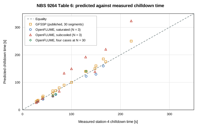
Figure 1. Predicted against measured station-4 chilldown time for all eighteen Table-6 rows: GFSSP's published predictions and OpenFLUME (N = 3; the four representative rows also at N = 30).
Representative subset at GFSSP's resolution
A saturated and a subcooled case of each fluid are solved at the refinement ladder N = 3, 6, 12, 30; N = 30 is GFSSP's resolution. The other fourteen rows are not solved above N = 3.
| Case | P_drive [psia] | Experiment [s] | GFSSP [s] | N = 3 | N = 6 | N = 12 | N = 30 |
|---|---|---|---|---|---|---|---|
| LN₂ saturated | 86.73 | 130 | 140 (+7.7 %) | 122.1 (−6.1 %) | 131.7 (+1.3 %) | 134.8 (+3.7 %) | 140.6 (+8.1 %) |
| LN₂ subcooled | 61.74 | 129 | 140 (+8.5 %) | 192.1 (+48.9 %) | 185.0 (+43.4 %)* | 207.4 (+60.8 %)* | — (—)* |
| LH₂ saturated | 74.97 | 68 | 70 (+2.9 %) | 55.9 (−17.8 %) | 56.2 (−17.3 %) | 56.6 (−16.8 %) | 57.4 (−15.6 %) |
| LH₂ subcooled | 86.73 | 62 | 60 (−3.2 %) | 51.1 (−17.6 %) | 51.6 (−16.8 %) | 51.0 (−17.7 %) | 51.6 (−16.7 %) |
| Four-row subset | n | MAE | Signed mean | Late | Range of errors |
|---|---|---|---|---|---|
| OpenFLUME, N = 3 | 4 | 22.6 % | +1.8 % | 1 | −17.8 % to +48.9 % |
| OpenFLUME, N = 6 | 4 | 19.7 % | +2.6 % | 2 | −17.3 % to +43.4 % |
| OpenFLUME, N = 12 | 4 | 24.8 % | +7.5 % | 2 | −17.7 % to +60.8 % |
| OpenFLUME, N = 30 | 3 | 13.5 % | −8.0 % | 1 | −16.7 % to +8.1 % |
| GFSSP (30 segments), published | 3 | 4.6 % | +2.5 % | 2 | −3.2 % to +8.5 % |
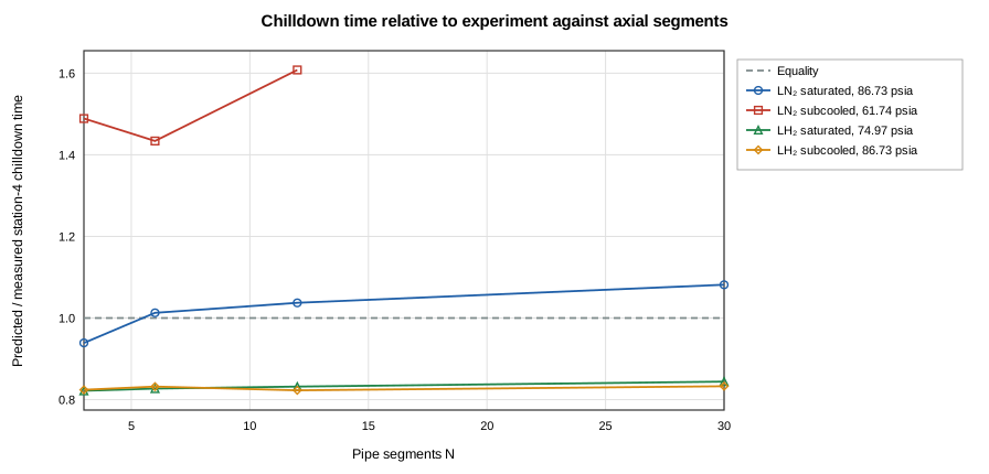
Figure 2. Predicted over measured station-4 chilldown time of the four representative cases against the number of axial segments.
Time-step sensitivity
The step used (Δt, 5 s for nitrogen and 1.25 s for hydrogen) is doubled and halved on the four representative cases at N = 3 (also quartered) and at N = 30 (a quarter step is not solved at N = 30); a solve is stopped after 390 s and listed with its partial history.
| Case | N | Δt × 2 | Δt (used) | Δt / 2 | Δt / 4 | |Δt − Δt/2| [s] | |Δt/2 − Δt/4| [s] | | ---- | - | ------ | --------- | ------ | ------ | ------------- | --------------- | | LN₂ saturated 86.73 | 3 | 119.6 | 122.1 | 119.2 | 119.2 | 2.9 | 0.0 | | LN₂ saturated 86.73 | 30 | 141.7 | 140.6 | 137.4 | not run | 3.2 | — | | LN₂ subcooled 61.74 | 3 | 196.6 | 192.1 | 213.0* | —* | 20.9 | — | | LN₂ subcooled 61.74 | 30 | 238.1 | —* | —* | not run | — | — | | LH₂ saturated 74.97 | 3 | 57.3 | 55.9 | 54.9 | 54.6 | 1.0 | 0.2 | | LH₂ saturated 74.97 | 30 | 59.4 | 57.4 | 56.6 | not run | 0.8 | — | | LH₂ subcooled 86.73 | 3 | 55.0 | 51.1 | 51.1* | 53.0* | 0.1 | 1.8 | | LH₂ subcooled 86.73 | 30 | 54.7 | 51.6 | 53.6 | not run | 1.9 | — |
(* : the solve did not converge; † : failed or timed out.) Between Δt and Δt/2 the chilldown time moves by at most 20.9 s at N = 3 and 3.2 s at N = 30 over the cases where both completed.
Not completed or not converged:
- LN₂ subcooled 61.74 psia, N = 3, Δt = 2.500 s: not converged
- LN₂ subcooled 61.74 psia, N = 3, Δt = 1.250 s: not converged
- LN₂ subcooled 61.74 psia, N = 30, Δt = 5.000 s: not converged
- LN₂ subcooled 61.74 psia, N = 30, Δt = 2.500 s: not converged
- LH₂ subcooled 86.73 psia, N = 3, Δt = 0.625 s: not converged
- LH₂ subcooled 86.73 psia, N = 3, Δt = 0.313 s: not converged
Longitudinal inertia
The four representative cases with and without the momentum-flux and kinetic-energy terms (longitudinalInertia), at N = 3 and N = 30:
| Case | P_drive [psia] | Experiment [s] | GFSSP [s] | No inertia, N = 3 | Inertia, N = 3 | No inertia, N = 30 | Inertia, N = 30 |
|---|---|---|---|---|---|---|---|
| LN₂ saturated | 86.73 | 130 | 140 | 113.5 (−12.7 %) | 122.1 (−6.1 %) | 134.9 (+3.8 %) | 140.6 (+8.1 %) |
| LN₂ subcooled | 61.74 | 129 | 140 | 175.4 (+36.0 %)* | 192.1 (+48.9 %) | 198.3 (+53.7 %)* | — (—)* |
| LH₂ saturated | 74.97 | 68 | 70 | 49.9 (−26.7 %) | 55.9 (−17.8 %) | 53.3 (−21.7 %) | 57.4 (−15.6 %) |
| LH₂ subcooled | 86.73 | 62 | 60 | 46.0 (−25.8 %)* | 51.1 (−17.6 %) | 47.7 (−23.1 %) | 51.6 (−16.7 %) |
Largest outlet-node Mach number at N = 30 (single-phase vapor steps):
| Case | P_drive [psia] | No inertia | Inertia |
|---|---|---|---|
| LN₂ saturated | 86.73 | 1.62 (> 1 for t = 80–105 s) | 0.71 |
| LN₂ subcooled | 61.74 | 1.27 (> 1 for t = 125–135 s) | 0.58 |
| LH₂ saturated | 74.97 | 1.73 (> 1 for t = 44–51 s) | 0.70 |
| LH₂ subcooled | 86.73 | 1.93 (> 1 for t = 34–45 s) | 0.72 |
Over all eighteen rows at N = 3 the mean absolute error is 24.1 % without the inertia terms and 19.3 % with them (18.1 % and 9.1 % without the subcooled LN₂ rows); the terms move the predicted time by −6.5 s to +24.9 s. Without inertia 6 rows are flagged.
Inlet restriction
Chilldown time of the subset at N = 3 against the inlet loss coefficient K (none: the 0.05 m negligible-friction inlet branch). [n]: number of stalled steps.
| Case | P_drive [psia] | Experiment [s] | No restriction | K = 1 | K = 2 (used) | K = 5 |
|---|---|---|---|---|---|---|
| LN₂ saturated | 86.73 | 130 | 121.8 (−6.3 %) | 121.9 (−6.2 %) | 122.1 (−6.1 %) | 122.4 (−5.8 %) |
| LN₂ subcooled | 61.74 | 129 | 183.3 (+42.1 %)* [2] | 201.2 (+56.0 %) | 192.1 (+48.9 %) | 183.8 (+42.5 %) |
| LH₂ saturated | 74.97 | 68 | 55.8 (−17.9 %) | 55.8 (−17.9 %) | 55.9 (−17.8 %) | 55.9 (−17.8 %) |
| LH₂ subcooled | 86.73 | 62 | 51.1 (−17.6 %) | 51.1 (−17.6 %) | 51.1 (−17.6 %) | 51.6 (−16.8 %) |
Between K = 1 and K = 5 the chilldown time moves by 0.5 s (LN₂ saturated), 17.4 s (LN₂ subcooled), 0.1 s (LH₂ saturated), 0.5 s (LH₂ subcooled). Over all eighteen rows at N = 3, 6 rows are flagged without the restriction and 3 with K = 2. Without it the first fluid node is held at the dewar pressure, where a subcooled inlet switches it between liquid and two-phase from one iteration to the next; the convection coefficient then jumps between Dittus–Boelter (of order 10³ W/m²K) and Miropolskii at low quality (of order 10 W/m²K), and the Newton iteration stalls.
Outlet pressure and the exit restriction
NBS 9264 and GFSSP give the outlet pressure as 12.05 psia (83.08 kPa; TFAWS 2013), and GFSSP's model has an exit restriction (Fig. 14 of AIAA 2015-3850) whose coefficient is not published. The subset at N = 3 with the outlet at 83.08 kPa and no exit restriction:
| Case | P_drive [psia] | Experiment [s] | GFSSP [s] | Outlet 101.325 kPa | Outlet 83.08 kPa |
|---|---|---|---|---|---|
| LN₂ saturated | 86.73 | 130 | 140 | 122.1 (−6.1 %) | 121.3 (−6.7 %) |
| LN₂ subcooled | 61.74 | 129 | 140 | 192.1 (+48.9 %) | 260.6 (+102.0 %)* |
| LH₂ saturated | 74.97 | 68 | 70 | 55.9 (−17.8 %) | 54.9 (−19.2 %) |
| LH₂ subcooled | 86.73 | 62 | 60 | 51.1 (−17.6 %) | 52.2 (−15.9 %)* |
The subcooled LN₂ case at 61.74 psia, station-4 knee and the state of the outlet fluid node (the node the outlet wall convects to) over the last 10 % of the solve:
| N | Outlet pressure [kPa] | Station-4 knee [s] | First liquid step at the outlet node [s] | Outlet node at the end |
|---|---|---|---|---|
| 3 | 101.325 | 192.1 (+48.9 %) | 235.0 | liquid |
| 3 | 83.08 (12.05 psia) | 260.6 (+102.0 %)* | never | twoPhase, x = 0.001–0.001 |
| 30 | 101.325 | not reached in 390 s* | never | vapor |
| 30 | 83.08 (12.05 psia) | not reached in 390 s* | never | vapor |
The subcooled LN₂ inlet (76 K) is saturated at 86.1 kPa. Near the outlet the line pressure approaches the boundary pressure, so below that pressure the liquid that reaches the outlet node cannot stay liquid: at 83.08 kPa the node stays two-phase at near-zero quality, where the Miropolskii coefficient is of order 10 W/m²K, instead of turning liquid (Dittus–Boelter, of order 10³ W/m²K). An exit restriction raises the outlet node's pressure above the boundary's; GFSSP's model has one, and its subcooled-LN₂ times are finite at 12.05 psia, which is consistent with a restriction that keeps that node liquid, but its coefficient is not published and this is not established here. At N = 30 neither outlet pressure gives a usable time: both solves accept stalled steps and station 4 does not reach the knee within the horizon (energy closure 153 % and 147 %). The subcooled LN₂ rows therefore depend on an unpublished input of GFSSP's model and are not quoted as point values.
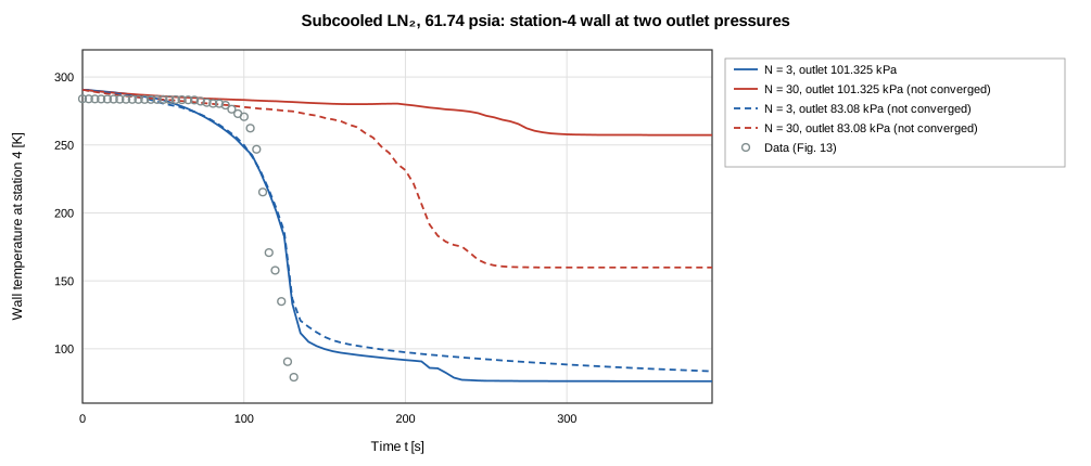
Figure 11. Subcooled LN₂ at 61.74 psia: station-4 wall temperature at N = 3 and N = 30 with the outlet at 101.325 kPa (solid) and 83.08 kPa (dashed), no exit restriction, against the digitized trace.
Knee of the digitized traces under the same definition
The threshold temperature of each digitized run's model solve (N = 3) is applied to the station-4 data trace of that run. The last column is the earlier data-native convention (T_inlet + 15 K), which sits above the unified threshold by the difference between the inlet liquid temperature and the local saturation temperature at the late-time pressure.
| Figure | P_drive [psia] | Table 6 [s] | Threshold [K] | Data knee | Model knee | Data knee at T_inlet + 15 K |
|---|---|---|---|---|---|---|
| Fig. 2 | 74.97 | 68 | 37.4 | 65.9 (−3.2 %) | 55.9 (−17.8 %) | 65.7 (−3.4 %) |
| Fig. 3 | 36.75 | 148 | 35.3 | 139.4 (−5.8 %) | 139.0 (−6.1 %) | 139.4 (−5.8 %) |
| Fig. 4 | 61.74 | 75 | 35.4 | 72.6 (−3.2 %) | 67.8 (−9.6 %) | 72.6 (−3.2 %) |
| Fig. 5 | 86.73 | 62 | 35.4 | 58.8 (−5.2 %) | 51.1 (−17.6 %) | 58.8 (−5.2 %) |
| Fig. 6 | 111.72 | 41 | 35.5 | 39.0 (−4.9 %) | 41.2 (+0.5 %) | not reached |
| Fig. 7 | 161.7 | 28 | 35.8 | 25.9 (−7.4 %) | 26.2 (−6.3 %) | 25.9 (−7.4 %) |
| Fig. 12 | 86.73 | 130 | 100.2 | 119.5 (−8.0 %) | 122.1 (−6.1 %) | 118.8 (−8.6 %) |
| Fig. 13 | 61.74 | 129 | 92.6 | 126.9 (−1.6 %) | 192.1 (+48.9 %) | 127.0 (−1.5 %) |
| Fig. 14 | 86.73 | 85 | 92.8 | 82.6 (−2.9 %) | 133.2 (+56.7 %) | 84.6 (−0.5 %) |
The data's knee under the identical definition is available for 9 of 9 digitized rows and differs from the tabulated chilldown time by −8.0 % to −1.6 %. The tabulated Table-6 times and the digitized knees are two readings of the same event, not independent constraints.
Sensitivity to the knee margin
The margin above T_sat,local is varied on the N = 3 solves of all rows.
| Fluid | P_drive [psia] | Experiment [s] | P_local,late [psia] | Threshold at 15 K [K] | T_sat,local + 15 K [s] | T_sat,local + 30 K [s] | Shift |
|---|---|---|---|---|---|---|---|
| LH₂ saturated | 74.97 | 68 | 26.06 | 37.4 | 55.9 | 55.1 | +0.7 s |
| LH₂ saturated | 86.73 | 62 | 28.73 | 37.8 | 49.5 | 48.7 | +0.8 s |
| LH₂ saturated | 111.72 | 42 | 34.32 | 38.5 | 38.5 | 38.1 | +0.4 s |
| LH₂ saturated | 161.72 | 30 | 44.93 | 39.7 | 28.2 | 27.6 | +0.7 s |
| LH₂ subcooled | 36.75 | 148 | 14.93 | 35.3 | 139.0 | 137.4 | +1.6 s |
| LH₂ subcooled | 61.74 | 75 | 15.19 | 35.4 | 67.8 | 66.3 | +1.5 s |
| LH₂ subcooled | 86.73 | 62 | 15.46 | 35.4 | 51.1 | 50.6 | +0.5 s |
| LH₂ subcooled | 111.72 | 41 | 15.74 | 35.5 | 41.2 | 40.6 | +0.6 s |
| LH₂ subcooled | 136.72 | 32 | 16.19 | 35.6 | 31.2 | 30.9 | +0.4 s |
| LH₂ subcooled | 161.7 | 28 | 16.97 | 35.8 | 26.2 | 25.8 | +0.4 s |
| LN₂ saturated | 61.74 | 165 | 26.69 | 97.8 | 159.3 | 145.3 | +14.0 s |
| LN₂ saturated | 74.97 | 150 | 30.53 | 99.1 | 129.4 | 118.8 | +10.6 s |
| LN₂ saturated | 86.73 | 130 | 33.91 | 100.2 | 122.1 | 113.1 | +9.0 s |
| LN₂ subcooled | 36.75 | 222 | 14.93 | 92.5 | 323.2 | 249.8 | +73.5 s |
| LN₂ subcooled | 49.97 | 170 | 15.07 | 92.6 | 220.0 | 211.7 | +8.3 s |
| LN₂ subcooled | 61.74 | 129 | 15.19 | 92.6 | 192.1 | 138.0 | +54.0 s |
| LN₂ subcooled | 74.97 | 100 | 15.33 | 92.7 | 149.4 | 146.3 | +3.2 s |
| LN₂ subcooled | 86.73 | 85 | 15.45 | 92.8 | 133.2 | 117.2 | +16.0 s |
Raising the margin from 15 K to 30 K moves the predicted time by +0.4 s to +73.5 s (+0.8 % to +41.9 % of the measured time).
Initial wall temperature: sensitivity
| Fluid | P_drive [psia] | T₀ used [K] | 300 K start | Measured T₀ start | Shift |
|---|---|---|---|---|---|
| LH₂ saturated | 74.97 | 280.3 | 59.7 (−12.3 %) | 55.9 (−17.8 %) | −3.8 s |
| LH₂ saturated | 86.73 | 287.6ᵃ | 51.1 (−17.5 %) | 49.5 (−20.2 %) | −1.6 s |
| LH₂ saturated | 111.72 | 287.6ᵃ | 40.2 (−4.2 %) | 38.5 (−8.2 %) | −1.7 s |
| LH₂ saturated | 161.72 | 287.6ᵃ | 29.4 (−2.2 %) | 28.2 (−5.9 %) | −1.1 s |
| LH₂ subcooled | 36.75 | 270.8 | 139.7 (−5.6 %)* | 139.0 (−6.1 %)* | −0.7 s |
| LH₂ subcooled | 61.74 | 276.7 | 74.8 (−0.3 %) | 67.8 (−9.6 %) | −7.0 s |
| LH₂ subcooled | 86.73 | 296.5 | 54.5 (−12.0 %)* | 51.1 (−17.6 %) | −3.4 s |
| LH₂ subcooled | 111.72 | 296.3 | 43.6 (+6.3 %)* | 41.2 (+0.5 %)* | −2.4 s |
| LH₂ subcooled | 136.72 | 287.6ᵃ | 32.5 (+1.5 %) | 31.2 (−2.4 %) | −1.3 s |
| LH₂ subcooled | 161.7 | 279.4 | 28.7 (+2.4 %) | 26.2 (−6.3 %) | −2.4 s |
| LN₂ saturated | 61.74 | 287.6ᵃ | 169.7 (+2.9 %) | 159.3 (−3.5 %) | −10.4 s |
| LN₂ saturated | 74.97 | 287.6ᵃ | 137.1 (−8.6 %) | 129.4 (−13.7 %) | −7.7 s |
| LN₂ saturated | 86.73 | 306.8 | 115.6 (−11.1 %) | 122.1 (−6.1 %) | +6.5 s |
| LN₂ subcooled | 36.75 | 287.6ᵃ | 383.7 (+72.9 %)* | 323.2 (+45.6 %)* | −60.5 s |
| LN₂ subcooled | 49.97 | 287.6ᵃ | 231.1 (+35.9 %)* | 220.0 (+29.4 %) | −11.0 s |
| LN₂ subcooled | 61.74 | 290.7 | 209.2 (+62.1 %) | 192.1 (+48.9 %) | −17.1 s |
| LN₂ subcooled | 74.97 | 287.6ᵃ | 153.7 (+53.7 %) | 149.4 (+49.4 %) | −4.3 s |
| LN₂ subcooled | 86.73 | 294.1 | 138.5 (+63.0 %) | 133.2 (+56.7 %) | −5.3 s |
With the 300 K start the mean absolute error at N = 3 is 20.8 % (signed mean +12.6 %); with the measured initial temperatures 19.3 % (+6.3 %). The shift in the predicted time is −60.5 s to +6.5 s. For the nine rows without a digitized run, the lowest and highest initial temperature of the corpus bracket the prediction (N = 3):
| Fluid | P_drive [psia] | T₀ = 270.8 K [s] | T₀ = 287.6 K [s] | T₀ = 306.8 K [s] | Spread [s] |
|---|---|---|---|---|---|
| LH₂ saturated | 86.73 | 46.3 | 49.5 | 52.3 | 6.0 |
| LH₂ saturated | 111.72 | 36.5 | 38.5 | 41.0 | 4.5 |
| LH₂ saturated | 161.72 | 26.8 | 28.2 | 29.7 | 2.9 |
| LH₂ subcooled | 136.72 | 29.9 | 31.2 | 33.7 | 3.8 |
| LN₂ saturated | 61.74 | 146.7 | 159.3 | 174.8 | 28.1 |
| LN₂ saturated | 74.97 | 119.0 | 129.4 | 140.4 | 21.5 |
| LN₂ subcooled | 36.75 | 327.4 | 323.2 | 378.5 | 51.1 |
| LN₂ subcooled | 49.97 | 204.4 | 220.0 | 243.4 | 39.0 |
| LN₂ subcooled | 74.97 | 138.9 | 149.4 | 164.2 | 25.3 |
The bracket spans 2.9 s to 51.1 s for these rows.
Layout
| Fluid | P_drive [psia] | Experiment [s] | Legacy layout, N = 3 | GFSSP layout, N = 3 |
|---|---|---|---|---|
| LH₂ saturated | 74.97 | 68 | 57.7 (−15.2 %) | 55.9 (−17.8 %) |
| LH₂ saturated | 86.73 | 62 | 51.0 (−17.8 %) | 49.5 (−20.2 %) |
| LH₂ saturated | 111.72 | 42 | 40.1 (−4.4 %) | 38.5 (−8.2 %) |
| LH₂ saturated | 161.72 | 30 | 29.9 (−0.4 %) | 28.2 (−5.9 %) |
| LH₂ subcooled | 36.75 | 148 | 133.3 (−9.9 %) | 139.0 (−6.1 %)* |
| LH₂ subcooled | 61.74 | 75 | 68.4 (−8.7 %) | 67.8 (−9.6 %) |
| LH₂ subcooled | 86.73 | 62 | 51.1 (−17.5 %) | 51.1 (−17.6 %) |
| LH₂ subcooled | 111.72 | 41 | 39.9 (−2.7 %) | 41.2 (+0.5 %)* |
| LH₂ subcooled | 136.72 | 32 | 32.3 (+0.9 %) | 31.2 (−2.4 %) |
| LH₂ subcooled | 161.7 | 28 | 27.2 (−2.9 %) | 26.2 (−6.3 %) |
| LN₂ saturated | 61.74 | 165 | 188.5 (+14.3 %) | 159.3 (−3.5 %) |
| LN₂ saturated | 74.97 | 150 | 160.3 (+6.9 %) | 129.4 (−13.7 %) |
| LN₂ saturated | 86.73 | 130 | 160.6 (+23.5 %) | 122.1 (−6.1 %) |
| LN₂ subcooled | 36.75 | 222 | 289.4 (+30.4 %) | 323.2 (+45.6 %)* |
| LN₂ subcooled | 49.97 | 170 | 202.1 (+18.9 %) | 220.0 (+29.4 %) |
| LN₂ subcooled | 61.74 | 129 | 159.1 (+23.3 %) | 192.1 (+48.9 %) |
| LN₂ subcooled | 74.97 | 100 | 127.6 (+27.6 %) | 149.4 (+49.4 %) |
| LN₂ subcooled | 86.73 | 85 | 112.2 (+32.1 %) | 133.2 (+56.7 %) |
With the legacy layout the N = 3 mean absolute error is 14.3 % (signed mean +5.4 %) against 19.3 % (+6.3 %) with GFSSP's layout. The legacy layout has no inlet branch, so it carries no inlet restriction; both include longitudinal inertia.
Subcooled liquid nitrogen
The subcooled liquid-nitrogen case at 61.74 psia has the largest error of the representative subset (192.1 (+48.9 %) at N = 3, 185.0 (+43.4 %)* at N = 6, 207.4 (+60.8 %)* at N = 12, — (—)* at N = 30; GFSSP +8.5 %). The diagnostics record the outlet fluid node (the one the outlet wall convects to), the heat the wall gives up by the phase of the fluid it is attached to, and the energy closure. The saturated case at 86.73 psia is the comparison. All solves are at the step used (Δt = 5 s).
| Case | N | Δt [s] | t(250 K) [s] | t(150 K) [s] | Knee [s] | First liquid at outlet node [s] | Minimum two-phase quality (wall < 150 K) | Minimum h, two-phase [W/m²K] | h at first liquid step [W/m²K] | Wall heat to vapor / two-phase / liquid [%] | Energy closure |
|---|---|---|---|---|---|---|---|---|---|---|---|
| subLN2-P61.74 | 3 | 5 | 98.8 | 128.3 | 192.1 | 235.0 | 0.000 | 24 | 6680 | 80 / 10 / 11 | 8.4 % |
| subLN2-P61.74 | 6* | 5 | 116.9 | 141.4 | 185.0 | 195.0 | 0.001 | 27 | 6557 | 76 / 9 / 15 | 1.7 % |
| subLN2-P61.74 | 12* | 5 | 146.1 | 161.0 | 207.4 | 210.0 | 0.001 | 28 | 6710 | 65 / 12 / 22 | 16.3 % |
| subLN2-P61.74 | 30* | 5 | — | — | — | never | — | — | — | 79 / 20 / 2 | 153.5 % |
| satLN2-P86.73 | 3 | 5 | 82.2 | 106.0 | 122.1 | never | 0.128 | 266 | — | 86 / 14 / 0 | 0.1 % |
| satLN2-P86.73 | 6 | 5 | 94.7 | 112.8 | 131.7 | never | 0.138 | 250 | — | 81 / 19 / 0 | 0.1 % |
| satLN2-P86.73 | 12 | 5 | 102.3 | 114.9 | 134.8 | never | 0.147 | 239 | — | 72 / 28 / 0 | 0.0 % |
| satLN2-P86.73 | 30 | 5 | 107.1 | 119.1 | 140.6 | never | 0.159 | 226 | — | 61 / 39 / 0 | -0.0 % |
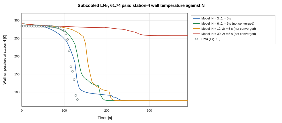
Figure 10. Subcooled LN₂ at 61.74 psia: station-4 wall temperature of the model at N = 3, 6, 12, 30 against the digitized Fig. 13 trace.
What the diagnostics show (a * on N marks a solve with stalled steps; its numbers are listed but not used in the statements below):
- Shelf and handoff. On the converged subcooled solves the outlet node's two-phase quality falls to 0.000 while the outlet wall is below 150 K (saturated case: 0.13–0.16). The Miropolskii coefficient falls with quality (
src/core/correlations/miropolskii.ts): its minimum is 24 W/m²K on the subcooled shelf against 226–266 W/m²K in the saturated case. When the outlet node turns single-phase liquid the conductor switches to Dittus–Boelter and h is 6680 W/m²K at the first liquid step, which comes +43 s relative to the station-4 knee of these solves; in the saturated case the outlet node never turns liquid. - The correlation as implemented is the documented one. Its coefficients (0.023, exponents 0.8 and 0.4, and the factor Y with 0.1, 0.4, 0.4) are those of Eq. 7h of the GFSSP manual, with Dittus–Boelter (Eq. 7g) on single-phase states, so the switch at the liquid boundary is the formulation's. Quality is clamped to [0.01, 0.99] inside the correlation. No change to the correlation was made.
- Refinement. The chilldown time of this case is 192.1 s (N = 3), 185.0 s* (N = 6), 207.4 s* (N = 12), — s* (N = 30); in the saturated case 122.1 s (N = 3), 131.7 s (N = 6), 134.8 s (N = 12), 140.6 s (N = 30). The interval from the outlet wall's 150 K arrival to the knee is 63.8 s (N = 3) for the subcooled case and 16.1 s, 18.9 s, 19.9 s, 21.5 s for the saturated one.
- Outlet pressure. The outlet node's phase, and with it the coefficient of the outlet wall, depends on the outlet pressure and on GFSSP's unpublished exit restriction ("Outlet pressure and the exit restriction"). The subcooled LN₂ times are therefore a sensitivity to that input, not point predictions.
Wall-temperature traces of the trusted runs
The 7 trusted runs are solved at N = 6 with the validation model, each from its measured initial wall temperature, with Δt = 5 s for nitrogen and 1.25 s for para-hydrogen (the frozen calibration plan, TRACE_BASELINE_SOLVE_PLAN, differs from these: Δt = 10 s and 2.5 s, 300 K start); subcooled runs start at their recorded inlet temperature. Model traces are interpolated to the exact station positions and aligned to the digitized record; nothing is tuned. The knee threshold is the unified one, from each solve's own late-time pressure. These numbers are reported, not gated.
| Run | Condition | Model | Converged | Pooled RMSE [K] | Pooled MAE [K] |
|---|---|---|---|---|---|
| Fig. 2 | saturated LH2, 5.1 atm | ParaHydrogen, N = 6, Δt = 1.25 s, T₀ = 280.3 K | yes | 68.0 | 47.0 |
| Fig. 5 | subcooled LH2, 5.9 atm | ParaHydrogen, N = 6, Δt = 1.25 s, T₀ = 296.5 K | yes | 63.7 | 38.4 |
| Fig. 10 | saturated LN2, 2.5 atm | Nitrogen, N = 6, Δt = 5 s, T₀ = 275.5 K | yes | 30.2 | 22.0 |
| Fig. 11 | saturated LN2, 3.4 atm | Nitrogen, N = 6, Δt = 5 s, T₀ = 296.6 K | yes | 34.9 | 27.8 |
| Fig. 12 | saturated LN2, 5.9 atm | Nitrogen, N = 6, Δt = 5 s, T₀ = 306.8 K | yes | 23.0 | 16.2 |
| Fig. 13 | subcooled LN2, 4.2 atm | Nitrogen, N = 6, Δt = 5 s, T₀ = 290.7 K | yes | 57.4 | 40.2 |
| Fig. 14 | subcooled LN2, 5.9 atm | Nitrogen, N = 6, Δt = 5 s, T₀ = 294.1 K | no | 72.3 | 52.7 |
| Run | Station | Knee threshold [K] | Data t(150 K) [s] | Model t(150 K) [s] | Data knee [s] | Model knee [s] | Knee lag | RMSE [K] |
|---|---|---|---|---|---|---|---|---|
| Fig. 2 | 1 | 42.0 | 9.3 | 13.1 | 19.9 | 30.2 | +10.3 s | 34.7 |
| Fig. 2 | 2 | 41.2 | 33.3 | 32.1 | 42.5 | 46.0 | +3.5 s | 33.3 |
| Fig. 2 | 3 | 39.8 | 55.0 | 45.5 | 63.9 | 53.9 | −10.0 s | 92.8 |
| Fig. 2 | 4 | 37.0 | 63.5 | 50.9 | 65.9 | 56.2 | −9.6 s | 128.1 |
| Fig. 5 | 1 | 42.4 | 9.5 | 12.1 | 18.4 | 26.1 | +7.7 s | 24.2 |
| Fig. 5 | 2 | 40.8 | 31.7 | 29.6 | 39.4 | 41.0 | +1.6 s | 35.2 |
| Fig. 5 | 3 | 38.6 | 49.9 | 41.4 | 56.3 | 48.7 | −7.7 s | 90.9 |
| Fig. 5 | 4 | 35.4 | 56.7 | 46.3 | 58.8 | 51.9 | −6.9 s | 153.1 |
| Fig. 10 | 1 | 100.8 | 68.9 | 81.7 | 83.9 | 294.9 | +211.0 s | 25.6 |
| Fig. 10 | 2 | 100.0 | 132.5 | 154.2 | 177.6 | 243.2 | +65.6 s | 33.8 |
| Fig. 10 | 3 | 98.2 | 188.1 | 213.1 | 213.7 | 269.1 | +55.5 s | 34.5 |
| Fig. 10 | 4 | 94.0 | 238.7 | 239.0 | — | — | — | 10.9 |
| Fig. 11 | 1 | 104.1 | 59.7 | 67.4 | — | 196.9 | — | 18.4 |
| Fig. 11 | 2 | 103.0 | 104.2 | 125.5 | — | 181.9 | — | 49.3 |
| Fig. 11 | 3 | 100.8 | 161.3 | 169.5 | — | 206.0 | — | 22.7 |
| Fig. 11 | 4 | 95.6 | 195.5 | 188.4 | 200.0 | 224.1 | +24.1 s | 41.7 |
| Fig. 12 | 1 | 110.8 | 36.9 | 41.3 | 44.0 | 88.5 | +44.5 s | 16.2 |
| Fig. 12 | 2 | 109.3 | 63.7 | 75.0 | 73.9 | 99.3 | +25.4 s | 29.2 |
| Fig. 12 | 3 | 106.5 | 102.0 | 101.1 | 115.3 | 119.0 | +3.7 s | 9.3 |
| Fig. 12 | 4 | 99.4 | 116.1 | 112.8 | 119.6 | 131.7 | +12.0 s | 31.4 |
| Fig. 13 | 1 | 105.7 | 19.9 | 39.9 | — | 60.0 | — | 59.9 |
| Fig. 13 | 2 | 102.5 | 65.1 | 93.4 | — | 116.3 | — | 66.7 |
| Fig. 13 | 3 | 98.3 | 96.8 | 130.5 | — | 148.5 | — | 60.5 |
| Fig. 13 | 4 | 92.6 | 120.9 | 139.3 | 126.9 | 184.0 | +57.1 s | 44.6 |
| Fig. 14 | 1 | 109.8 | 14.5 | 33.0 | — | 48.9 | — | 56.2 |
| Fig. 14 | 2 | 105.9 | 34.9 | 69.9 | — | 82.8 | — | 96.8 |
| Fig. 14 | 3 | 100.6 | 65.6 | 90.5 | 87.0 | 104.2 | +17.2 s | 75.4 |
| Fig. 14 | 4 | 92.8 | 78.0 | 100.7 | 82.6 | 139.1 | +56.6 s | 54.4 |
(N = 6; — : the feature is unavailable — the trace never reaches it inside the record, or the data trace's cold tail is QC-excluded.)
Observations (computed from the tables; the figures overlay model and data). Pooled RMSE at N = 6 is 23.0–68.0 K for the saturated runs and 57.4–72.3 K for the subcooled ones.
- Station 1 (6.1 m, N = 6, all trusted runs). The modeled wall reaches the unified knee threshold inside the record in 7 of 7 runs (the data trace does in 4). Where both knees exist the model's is +7.7 s to +211.0 s from the measured one (4 later, 0 earlier of 4). The 150 K arrival at station 1 differs by +2.5 s to +20.0 s; the first 30 K of cooling (the leading edge) by −1.1 s to +5.4 s.
- Station 4 (60.35 m). Where both knees exist the model's is −9.6 s to +57.1 s from the measured one (4 later, 2 earlier of 6); the leading edge differs by −27.1 s to +10.9 s.
- 150 K arrivals at stations 2–4. The modeled arrival is later than the measured one in 12 and earlier in 9 of 21 station pairs (range −12.6 s to +35.0 s). The model and the data order the stations' arrivals identically in 7 of 7 runs.
- Front width at station 4 (time from 250 K to the knee threshold): model 21.7, 17.4, —, 60.1, 36.9, 62.2, 55.5 s against data 7.2, 5.3, —, 14.1, 9.3, 19.8, 12.6 s (— : not available, the data trace's cold tail is QC-excluded or a threshold is not reached). Where both exist the model/data ratio is 3.0–4.4.
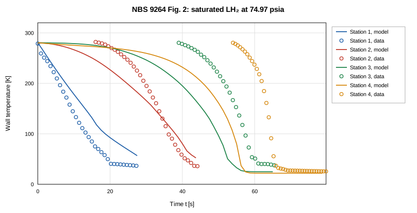
Figure 3. Fig. 2 of NBS 9264 (saturated LH₂, 5.1 atm): digitized wall temperature (markers) and the OpenFLUME solve (lines, N = 6, Δt = 1.25 s, T₀ = 280.3 K) at the four stations.
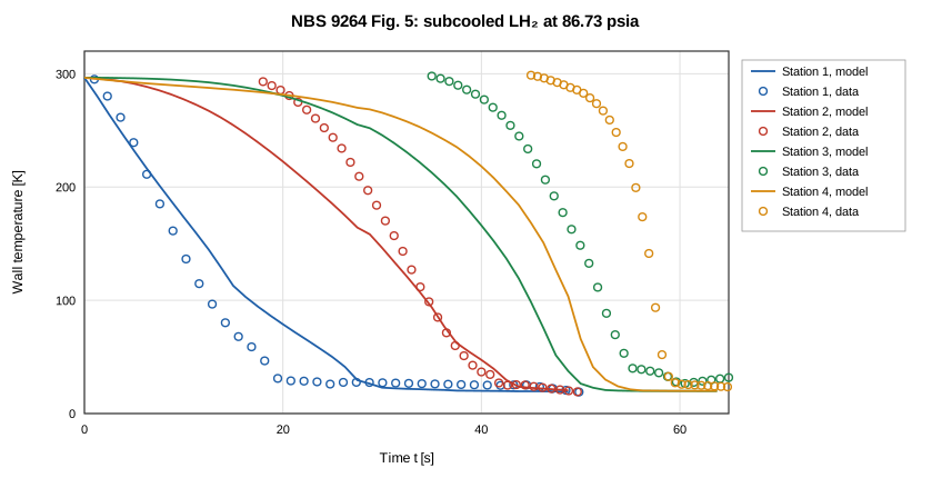
Figure 4. Fig. 5 of NBS 9264 (subcooled LH₂, 5.9 atm): digitized wall temperature (markers) and the OpenFLUME solve (lines, N = 6, Δt = 1.25 s, T₀ = 296.5 K) at the four stations.
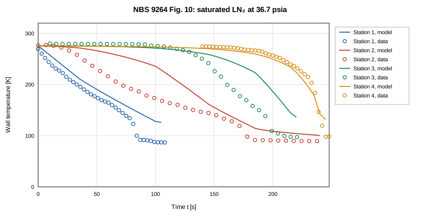
Figure 5. Fig. 10 of NBS 9264 (saturated LN₂, 2.5 atm): digitized wall temperature (markers) and the OpenFLUME solve (lines, N = 6, Δt = 5 s, T₀ = 275.5 K) at the four stations.
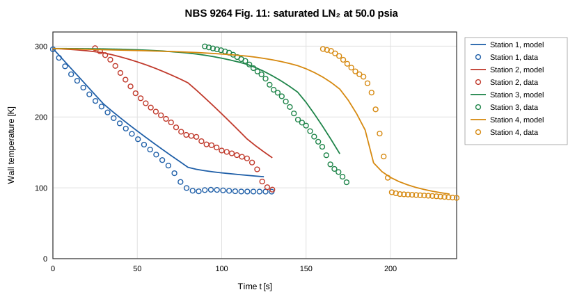
Figure 6. Fig. 11 of NBS 9264 (saturated LN₂, 3.4 atm): digitized wall temperature (markers) and the OpenFLUME solve (lines, N = 6, Δt = 5 s, T₀ = 296.6 K) at the four stations.
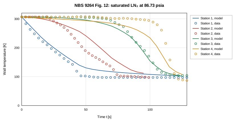
Figure 7. Fig. 12 of NBS 9264 (saturated LN₂, 5.9 atm): digitized wall temperature (markers) and the OpenFLUME solve (lines, N = 6, Δt = 5 s, T₀ = 306.8 K) at the four stations.
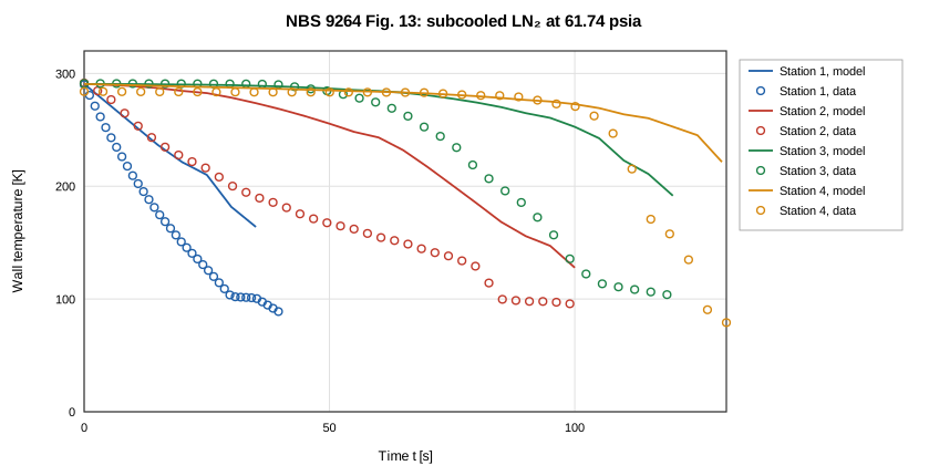
Figure 8. Fig. 13 of NBS 9264 (subcooled LN₂, 4.2 atm): digitized wall temperature (markers) and the OpenFLUME solve (lines, N = 6, Δt = 5 s, T₀ = 290.7 K) at the four stations.
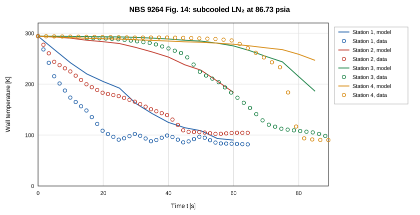
Figure 9. Fig. 14 of NBS 9264 (subcooled LN₂, 5.9 atm): digitized wall temperature (markers) and the OpenFLUME solve (lines, N = 6, Δt = 5 s, T₀ = 294.1 K) at the four stations.
Solves that failed or did not converge
dt|subLH2-P86.73|N3|P|dt0.3125: 78 stalled step(s)t6|subLN2-P61.74|N30|P: 71 stalled step(s)t6|subLN2-P61.74|N30|NOI: 2 stalled step(s)t6|subLN2-P61.74|N12|P: 6 stalled step(s)dt|subLH2-P86.73|N3|P|dt0.625: 21 stalled step(s)t6|subLH2-P36.75|N3|T300: 20 stalled step(s)t6|subLH2-P36.75|N3|P: 50 stalled step(s)t6|subLH2-P36.75|N3|NOI: 41 stalled step(s)t6|subLH2-P36.75|N3|NOK: 49 stalled step(s)dt|subLN2-P61.74|N3|P|dt1.25: 280 stalled step(s)t6|subLN2-P61.74|N6|P: 1 stalled step(s)t6|subLH2-P86.73|N3|NOI: 1 stalled step(s)t6|subLH2-P86.73|N3|T300: 3 stalled step(s)t6|subLH2-P111.72|N3|P: 1 stalled step(s)t6|subLH2-P111.72|N3|T300: 4 stalled step(s)t6|subLH2-P111.72|N3|NOK: 2 stalled step(s)t6|subLH2-P86.73|N3|P83: 1 stalled step(s)t6|subLN2-P36.75|N3|P: 4 stalled step(s)t6|subLN2-P36.75|N3|T300: 3 stalled step(s)t6|subLN2-P36.75|N3|NOI: 2 stalled step(s)dt|subLN2-P61.74|N3|P|dt2.5: 38 stalled step(s)t6|subLN2-P36.75|N3|TLO: 1 stalled step(s)t6|subLN2-P36.75|N3|NOK: 12 stalled step(s)tr|nbs9264-fig14|N6|P: 1 stalled step(s)t6|subLN2-P49.97|N3|T300: 1 stalled step(s)t6|subLN2-P36.75|N3|THI: 10 stalled step(s)t6|subLN2-P49.97|N3|NOK: 3 stalled step(s)t6|subLN2-P49.97|N3|TLO: 1 stalled step(s)t6|subLN2-P49.97|N3|NOI: 3 stalled step(s)t6|subLN2-P61.74|N3|NOI: 1 stalled step(s)t6|subLN2-P61.74|N3|P83: 5 stalled step(s)t6|subLN2-P61.74|N3|NOK: 2 stalled step(s)t6|subLN2-P74.97|N3|NOI: 3 stalled step(s)t6|subLN2-P74.97|N3|NOK: 3 stalled step(s)t6|subLN2-P61.74|N30|P83: 60 stalled step(s)dt|subLN2-P61.74|N30|P|dt2.5: stopped at the 390 s limit at t = 332.5 s, 0 stalled step(s)
Trust Levels
| Comparison | Evidence class | Trust level | What may be quoted |
|---|---|---|---|
| Table-6 rows without a compromised record (14 rows) | Validation against experiment | Trusted | The error, with the definition, initial temperature and discretization stated |
| Table-6 rows whose digitized record is compromised (4 rows) | Validation against experiment | Diagnostic only | The trend; the error with that caveat |
| GFSSP Table-6 predictions | Code-to-code | Reference | Agreement between codes, not with experiment |
| Rows with stalled steps (3 at N = 3) | Validation against experiment | Flagged | The time with the flag; excluded from the summary statistics |
| Subcooled LN₂ rows | Validation against experiment | Sensitive to an unpublished input (GFSSP's exit restriction, outlet pressure) | That the time depends on the outlet node's phase; not a point estimate |
| Trusted trace runs (Figs. 2, 5, 10, 11, 12, 13, 14) | Validation against experiment | Trusted, reported (not gated) | Station order, knees where available, RMSE as a baseline |
| Diagnostic trace runs (Figs. 3, 4, 6, 7) | Validation against experiment | Diagnostic only | Nothing quantitative |
Conclusions
Over all eighteen NBS 9264 Table-6 chilldown times, OpenFLUME's untuned two-phase network model, with GFSSP's longitudinal inertia term and an inlet restriction, has a mean absolute error of 19.3 % at the CI configuration (signed mean +6.3 %, 6 of 18 late), against 7.6 % for GFSSP's published predictions (+7.3 %, 16 late). Without the 3 flagged rows it is 19.7 % (GFSSP 7.6 %), and without the subcooled LN₂ rows as well 10.1 % over 11 rows (GFSSP 8.7 %). At GFSSP's resolution the 3 subset cases whose station 4 reaches the knee have a mean absolute error of 13.5 % (GFSSP 4.6 %; the four cases at N = 3: 22.6 %). The subcooled liquid-nitrogen rows are late; their outlet wall waits on a near-zero-quality film-boiling shelf, and whether the outlet node turns liquid depends on the outlet pressure and on GFSSP's unpublished exit restriction. The remaining difference from GFSSP on the hydrogen rows is not explained here; GFSSP's unpublished inputs (the valve and exit-restriction coefficients, the wall roughness, the copper properties below 100 K) are candidates. The chilldown-time comparison also depends on the initial wall temperature (−60.5 s to +6.5 s between a 300 K and the measured start) and on the knee margin (+0.8 % to +41.9 % for 15 K against 30 K). Cryogenic chilldown remains the least mature capability of the code, and these results are a baseline for model improvement, not a calibration.
References
- Brennan, J. A., Brentari, E. G., Smith, R. V., and Steward, W. G., "Cooldown of Cryogenic Transfer Lines — An Experimental Report," NBS Report 9264, National Bureau of Standards, Boulder CO, 1966 (NASA-CR-81338, NTRS 19670007291).
- Majumdar, A., LeClair, A., Moore, R., and Schallhorn, P., "Generalized Fluid System Simulation Program (GFSSP) Version 6," AIAA 2015-3850, 51st AIAA/SAE/ASEE Joint Propulsion Conference, 2015 (NTRS 20150016531), §4.3 and Table 6.
- Majumdar, A., "No Vent Tank Fill and Transfer Line Chilldown Analysis by Generalized Fluid System Simulation Program (GFSSP)," TFAWS 2013 (NASA M13-2805).
- Miropolskii, Z. L., "Heat Transfer in Film Boiling of a Steam–Water Mixture in Steam-Generating Tubes," Teploenergetika 10(5), 1963, pp. 49–52, as used for chilldown by Cross, M. F., Majumdar, A. K., Bennett, J. C., and Malla, R. B., "Modeling of Chill Down in Cryogenic Transfer Lines," Journal of Spacecraft and Rockets 39(2), 2002, pp. 284–289 (Eq. 17: the momentum equation with the longitudinal inertia term).
- NIST Cryogenic Material Properties Database, "OFHC Copper (UNS C10100/C10200)," rev. 2010 (Marquardt, Le, and Radebaugh, 2000).
Nomenclature
| Symbol | Meaning |
|---|---|
| MAE | mean absolute error |
| N | number of axial pipe segments |
| P_drive | dewar (driving) pressure |
| P_local,late | pressure at a station, mean over the final 10 % of the solve |
| RMSE | root-mean-square error between aligned traces |
| t(150 K) | first smooth crossing of 150 K |
| T₀ | initial wall temperature |
| T_inlet | inlet liquid temperature |
| T_sat, T_sat,local | saturation temperature; at the station's late-time pressure |
| Δt | solver time step |