
Steady Incompressible Network Hydraulics Validation of OpenFLUME
A validation report for the pressure–flow network solver against the classical closed-form results of steady incompressible pipe hydraulics: Hagen–Poiseuille laminar flow, Darcy–Weisbach turbulent flow, parallel-pipe flow splits, multi-loop network analysis (Hardy-Cross reference problem), hydrostatics, and pump/system operating points.
Generated by scripts/hydraulics-validation-report.ts — all numbers and figures come from live solves of the current solver. The corresponding CI gates are src/core/__tests__/solver.test.ts and src/core/__tests__/benchmarks.test.ts.
Abstract
This report verifies the steady incompressible-flow capability of the OpenFLUME solver — a pressure-based node-and-branch network code in the GFSSP family — against six benchmark problems of classical pipe hydraulics, each of which admits either an exact closed-form solution or an independent reference solution converged in this script to a tolerance far below the solver's own. The cases cover the laminar friction law (Hagen–Poiseuille), the turbulent Darcy–Weisbach law with a prescribed friction factor, the flow split among parallel pipes of unequal geometry, a six-node twelve-branch multi-loop water network of the kind classically solved with the Hardy-Cross method, hydrostatic pressure distributions with and without through-flow, and the operating point of a pump run against a pipe system curve. Across all 49 compared quantities the numerical solution reproduces the reference to within 9.98e-10 % — the agreement is limited only by the Newton convergence tolerance (10⁻⁹), not by any modeling approximation, because every case is constructed so that the solver's friction closure and the analytic reference are the same expression.
Introduction
Before a network flow solver can be trusted on problems without known answers, it must reproduce the problems with known answers. For steady incompressible flow the canonical set is small and sharp: the laminar Hagen–Poiseuille law (an exact solution of the Navier–Stokes equations), the Darcy–Weisbach equation with prescribed friction factor, mass-conservative flow splits, Kirchhoff-consistent loop networks — the problem class Hardy Cross's 1936 moment-distribution analogue was invented for — the hydrostatic law, and the intersection of a pump curve with a system curve. This report exercises the OpenFLUME steady solver on all six, mirroring the network configurations of the CI test suite (solver.test.ts, benchmarks.test.ts) so the report and the CI gates validate the same physics. The companion report (compressible-report.md) covers the compressible quasi-1-D capability; this one establishes the incompressible foundation underneath it.
Problem Description
The working fluid throughout is water, treated as an incompressible liquid (ρ = 998 kg/m³, μ = 0.001 Pa·s, the solver's water preset). Six cases are studied:
| Case | Description |
|---|---|
| 1 | Laminar flow in a small-bore pipe — ṁ vs ΔP against Hagen–Poiseuille, Re 200–1800 |
| 2 | Turbulent flow with fixed Darcy friction factor — ṁ vs ΔP over a ΔP decade |
| 3 | Flow split among three parallel pipes of unequal D, L, and f |
| 4 | Multi-loop water network: 6 internal nodes, 12 square-law resistances, 4 loops |
| 5 | Hydrostatics: a 20 m static water column, and a flowing inclined riser |
| 6 | Pump operating point: pump curve vs pipe system curve between equal reservoirs |
Cases 1, 2, 3, and 5 use pressure boundary pairs with pipe branches sized in the script; case 4 uses the multi-loop geometry of benchmark B1 in benchmarks.test.ts, shown in Figure 1; case 6 uses the pump curve of benchmark B2 discharging through a fixed-friction pipe with a 5 m static lift.

Figure 1. Topology of the multi-loop water network (case 4): two pressure boundaries at 500 kPa and 100 kPa, six internal nodes, twelve square-law resistance branches forming four independent loops.
Benchmark Solutions
Hagen–Poiseuille (case 1). For fully developed laminar flow the Darcy friction factor is exactly f = 64/Re, which turns the Darcy–Weisbach equation into the linear Hagen–Poiseuille law:
$$\Delta P = \frac{128,\mu L,\dot m}{\pi \rho D^4}, \qquad \dot m = \frac{\pi \rho D^4 \Delta P}{128,\mu L}.$$
Darcy–Weisbach with fixed f (case 2). With a prescribed constant friction factor the momentum balance closes exactly:
$$\Delta P = f,\frac{L}{D},\frac{\rho V^2}{2}, \qquad \dot m = A\sqrt{\frac{2\rho,\Delta P}{f L/D}}.$$
Parallel-pipe split (case 3). Parallel branches between common nodes see the same ΔP, so each branch flow follows the fixed-f closed form independently and the total is their sum:
$$\dot m_i = A_i\sqrt{\frac{2\rho,\Delta P, D_i}{f_i L_i}}, \qquad \dot m_{tot} = \sum_i \dot m_i.$$
Multi-loop network (case 4). Each branch is a square-law resistance ΔP = R·ṁ|ṁ| with R = K/(2ρA²). The network solution must satisfy Kirchhoff's two laws — mass continuity at every node and zero signed ΔP around every loop:
$$\sum_{j \in node} \dot m_j = 0, \qquad \sum_{j \in loop} \pm R_j,\dot m_j |\dot m_j| = 0.$$
This is the problem class of Cross (1936), whose iterative loop-correction scheme $$\Delta Q = -\frac{\sum_j \pm R_j Q_j |Q_j|}{2 \sum_j R_j |Q_j|}$$ predates but is equivalent in fixed point to a Newton iteration on the network equations. The reference here is an independent Newton solve of the nodal continuity equations with the exact branch law, implemented in this script with a finite-difference Jacobian and dense Gaussian elimination, converged to a mass residual below 10⁻¹² kg/s (18 iterations).
Hydrostatics (case 5). For a static column of incompressible liquid the pressure varies linearly with elevation,
$$P(z) = P_0 - \rho g z,$$
and for a flowing inclined pipe the boundary pressure difference splits into hydrostatic and frictional parts:
$$P_{bot} - P_{top} = \rho g,\Delta z + f,\frac{L}{D},\frac{\rho V^2}{2}.$$
Pump operating point (case 6). Between reservoirs of equal pressure, the steady flow settles where the pump pressure rise equals the system demand,
$$\Delta P_{pump}(\dot m) = \rho g,\Delta z + f,\frac{L}{D},\frac{\rho V^2}{2},$$
with the pump curve interpolated piecewise-linearly in volumetric flow Q = ṁ/ρ, exactly as the solver's pump component defines it. The reference operating point is found by bisection on this scalar equation to a bracket width of 10⁻¹² kg/s.
Numerical Modeling
OpenFLUME employs a finite volume formulation of the mass, momentum, and energy conservation equations on a network of nodes and branches: mass (and energy) conservation is enforced at every internal node, and each branch supplies one momentum relation between its endpoint pressures and its mass flow rate, solved as a coupled Newton system with pressure boundary conditions at boundary nodes. The flow rate is never prescribed — it is computed from the imposed pressures, exactly as in GFSSP.
The component physics exercised here:
pipeapplies the Darcy–Weisbach relation. With nofrictionFactoroverride the friction factor is f = 64/Re for Re < 2300 (exact Hagen–Poiseuille), the Swamee–Jain explicit Colebrook approximation for Re > 4000, and a C¹ smoothstep blend between (case 1 stays entirely below Re 1800, inside the exact laminar branch). WithfrictionFactorset, that constant f is used at every Reynolds number (cases 2, 3, 5b, 6), making the analytic references exact closures of the solver's own momentum equation. The pipe'selevationChangeadds the hydrostatic term ρg·Δz with g = 9.80665 m/s².resistanceapplies the square law ΔP = K·ṁ|ṁ|/(2ρA²) (case 4).pumpapplies a pressure rise interpolated piecewise-linearly from its (Q, ΔP) curve (case 6).
All solves use tolerance 10⁻⁹, maxIterations 500, and relaxation 0.9 (0.8 for the multi-loop network, matching benchmark B1). The compressible opt-in terms (momentumFlux, kineticEnergy) are left off: both are identically zero for constant-density flow. Internal nodes carry initial pressure guesses only; these do not constrain the converged solution.
Results and Discussion
Every case converged. The table summarizes the maximum relative deviation of each compared quantity from its reference; the errors sit at the Newton convergence floor (10⁻⁹ relative residual), orders of magnitude below any physical-modeling tolerance.
| Case | Compared quantity | Points | Max error |
|---|---|---|---|
| 1 — Laminar pipe | ṁ vs Hagen–Poiseuille | 9 | 9.98e-10 % |
| 2 — Turbulent pipe | ṁ vs Darcy–Weisbach | 8 | 5.36e-12 % |
| 3 — Parallel split | branch ṁ vs closed form | 3 | 5.62e-13 % |
| 3 — Parallel split | total ṁ | 1 | 3.43e-13 % |
| 4 — Multi-loop | branch ṁ vs independent Newton | 12 | 1.25e-12 % |
| 4 — Multi-loop | node P vs independent Newton | 6 | 4.57e-13 % |
| 5a — Static column | node P vs P₀ − ρgz | 9 | 0.00e+0 % of ρgH |
| 5b — Flowing riser | ṁ vs friction + ρgΔz closure | 1 | 1.82e-13 % |
| 6 — Pump | operating-point ṁ | 1 | 1.88e-13 % |
| 6 — Pump | operating-point rise | 1 | 1.72e-13 % |
Case 1: Laminar Pipe Flow (Hagen–Poiseuille)
A D = 10 mm, L = 10 m water pipe is driven by boundary-pressure pairs chosen to sweep the Reynolds number from 200 to 1800 — entirely inside the laminar regime, where the solver's friction factor is exactly 64/Re and the Hagen–Poiseuille law is an exact closure. Figure 2 shows the solved mass flow against the analytic line: ṁ is linear in ΔP, and the maximum deviation over the 9-point sweep is 9.98e-10 %. The solver-reported Reynolds numbers confirm every point sits below the laminar cutoff (Re = 2300), so no transition blending contaminates the comparison.
| ΔP [kPa] | ṁ analytic [kg/s] | ṁ numerical [kg/s] | Re | ṁ error |
|---|---|---|---|---|
| 0.064 | 1.57080e-3 | 1.57080e-3 | 200 | 9.98e-10 % |
| 0.128 | 3.14159e-3 | 3.14159e-3 | 400 | 4.57e-10 % |
| 0.192 | 4.71239e-3 | 4.71239e-3 | 600 | 4.57e-10 % |
| 0.257 | 6.28319e-3 | 6.28319e-3 | 800 | 6.23e-11 % |
| 0.321 | 7.85398e-3 | 7.85398e-3 | 1000 | 6.50e-11 % |
| 0.385 | 9.42478e-3 | 9.42478e-3 | 1200 | 5.24e-11 % |
| 0.449 | 1.09956e-2 | 1.09956e-2 | 1400 | 4.60e-11 % |
| 0.513 | 1.25664e-2 | 1.25664e-2 | 1600 | 3.90e-11 % |
| 0.577 | 1.41372e-2 | 1.41372e-2 | 1800 | 2.72e-11 % |
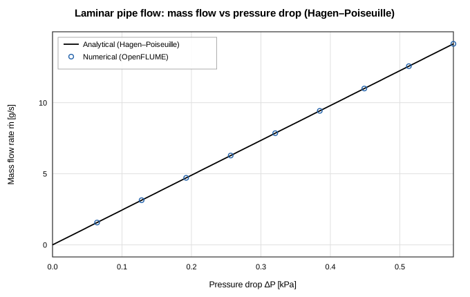
Figure 2. Laminar pipe flow: solved mass flow rate vs pressure drop against the exact Hagen–Poiseuille line.
Case 2: Turbulent Pipe Flow (Darcy–Weisbach)
A D = 50 mm, L = 10 m pipe with a prescribed constant friction factor f = 0.02 is swept over a ΔP decade (5–100 kPa). Because f is fixed, the Darcy–Weisbach inversion ṁ = A√(2ρΔP/(fL/D)) is exact, and the solved flow follows the square-root curve of Figure 3 to within 5.36e-12 %. Reynolds numbers span 7.9e+4 to 3.5e+5, comfortably turbulent.
| ΔP [kPa] | ṁ analytic [kg/s] | ṁ numerical [kg/s] | Re | ṁ error |
|---|---|---|---|---|
| 5.000 | 3.10145e+0 | 3.10145e+0 | 78978 | 2.42e-12 % |
| 7.671 | 3.84146e+0 | 3.84146e+0 | 97822 | 5.36e-12 % |
| 11.768 | 4.75802e+0 | 4.75802e+0 | 121162 | 1.14e-12 % |
| 18.053 | 5.89328e+0 | 5.89328e+0 | 150071 | 2.86e-13 % |
| 27.696 | 7.29941e+0 | 7.29941e+0 | 185878 | 6.94e-13 % |
| 42.489 | 9.04105e+0 | 9.04105e+0 | 230228 | 1.77e-13 % |
| 65.184 | 1.11982e+1 | 1.11982e+1 | 285161 | 3.49e-13 % |
| 100.000 | 1.38701e+1 | 1.38701e+1 | 353200 | 7.68e-14 % |
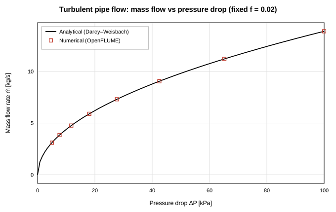
Figure 3. Turbulent pipe flow with fixed friction factor: solved mass flow rate vs pressure drop against the exact Darcy–Weisbach inversion.
Case 3: Parallel-Pipe Flow Split
Three pipes of unequal diameter, length, and friction factor connect the same two pressure boundaries (ΔP = 50 kPa). Each branch must carry ṁᵢ = Aᵢ√(2ρΔP·Dᵢ/(fᵢLᵢ)) independently; the solver reproduces every branch flow to within 5.62e-13 % and the total to within 3.43e-13 % (Figure 4). This exercises simultaneous momentum closure on parallel paths — the degenerate two-node limit of a loop network.
| Branch | D [mm] | L [m] | f | ṁ analytic [kg/s] | ṁ numerical [kg/s] | error |
|---|---|---|---|---|---|---|
| p1 | 40 | 8 | 0.02 | 6.276899 | 6.276899 | 1.41e-14 % |
| p2 | 60 | 12 | 0.025 | 12.632016 | 12.632016 | 5.62e-13 % |
| p3 | 25 | 6 | 0.03 | 1.827549 | 1.827549 | 0.00e+0 % |
| total | — | — | — | 20.736463 | 20.736463 | 3.43e-13 % |

Figure 4. Parallel-pipe flow split: analytic vs numerical branch flows for three unequal pipes at common ΔP.
Case 4: Multi-Loop Water Network (Hardy-Cross Reference)
The six-node, twelve-branch, four-loop network of Figure 1 (the geometry of CI benchmark B1) is driven from 500 kPa to 100 kPa through square-law resistances. The reference solution is this script's own Newton iteration on the nodal continuity equations with the exact branch law, converged to a mass residual below 10⁻¹² kg/s in 18 iterations. All twelve solver branch flows agree with the reference to within 1.25e-12 %, and all six internal node pressures to within 4.57e-13 % (Figure 5). As an internal-consistency check, the signed pressure-drop sums around the four independent loops of the solved network close to within 2.2e-16 of the 400 kPa system ΔP — Kirchhoff's second law is satisfied to solver precision.
| Branch | K | ṁ reference [kg/s] | ṁ solver [kg/s] | error |
|---|---|---|---|---|
| b1 (HP→N1) | 10 | 6.607218 | 6.607218 | 2.69e-13 % |
| b2 (N1→N2) | 5 | 5.610671 | 5.610671 | 1.20e-12 % |
| b3 (N2→LP) | 10 | 4.521599 | 4.521599 | 2.55e-13 % |
| b4 (HP→N3) | 8 | 7.403880 | 7.403880 | 2.40e-13 % |
| b5 (N3→N4) | 6 | 5.128094 | 5.128094 | 1.20e-12 % |
| b6 (N4→LP) | 8 | 5.025888 | 5.025888 | 2.30e-13 % |
| b7 (N3→N5) | 10 | 3.272332 | 3.272332 | 1.25e-12 % |
| b8 (N5→N6) | 5 | 3.272332 | 3.272332 | 1.00e-12 % |
| b9 (N6→LP) | 10 | 4.463610 | 4.463610 | 2.79e-13 % |
| b10 (N1→N3) | 2 | 0.996547 | 0.996547 | 1.78e-13 % |
| b11 (N2→N4) | 2 | 1.089072 | 1.089072 | 2.85e-13 % |
| b12 (N4→N6) | 2 | 1.191278 | 1.191278 | 5.41e-13 % |
| Node | P reference [kPa] | P solver [kPa] | error |
|---|---|---|---|
| N1 | 281.286 | 281.286 | 4.55e-13 % |
| N2 | 202.429 | 202.429 | 2.73e-13 % |
| N3 | 280.291 | 280.291 | 4.57e-13 % |
| N4 | 201.241 | 201.241 | 2.75e-13 % |
| N5 | 226.643 | 226.643 | 1.28e-14 % |
| N6 | 199.819 | 199.819 | 2.91e-13 % |
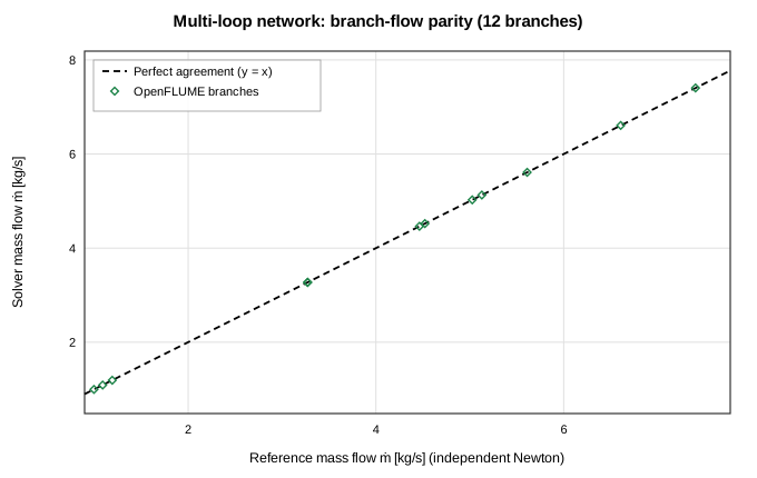
Figure 5. Multi-loop network: parity of solver branch flows against the independent Newton reference — all 12 branches on the y = x line.
Case 5: Hydrostatics
Static column. A 20 m vertical water column is discretized into 10 pipe segments with elevationChange set, and the two boundary pressures are placed in exact hydrostatic balance (P₀ = 300 kPa at the bottom, 104.26 kPa at the top). The solver recovers the linear pressure profile P = P₀ − ρgz at every interior node to within 0.00e+0 Pa (0.00e+0 % of the ρgH = 195.7 kPa column span), with a residual through-flow of 3.44e-13 kg/s — numerically zero (Figure 6).
Flowing inclined riser. A 20 m fixed-f pipe rising Δz = 5 m carries flow driven by a boundary ΔP composed of ρgΔz = 48.94 kPa of hydrostatic head plus 30 kPa of friction. The solver must superpose both momentum terms correctly to recover the closed-form flow: it returns ṁ = 5.371874 kg/s against the analytic 5.371874 kg/s, an error of 1.82e-13 %.
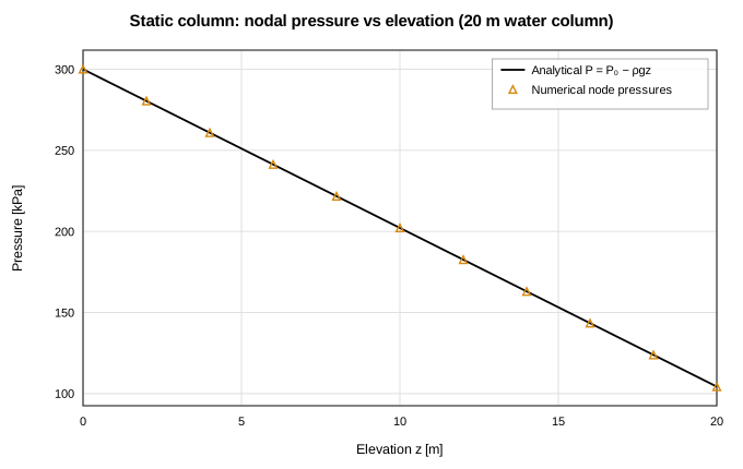
Figure 6. Static water column: solved nodal pressures vs the analytic hydrostatic line P = P₀ − ρgz.
Case 6: Pump Operating Point
The benchmark-B2 pump curve (200 kPa at 0 m³/s, 150 kPa at 0.01 m³/s, 50 kPa at 0.02 m³/s; piecewise linear in volumetric flow) discharges through a D = 50 mm, L = 10 m fixed-f pipe with a 5 m static lift, between reservoirs of equal pressure. The analytic operating point — the intersection of the pump curve with the system curve ρgΔz + f(L/D)ρV²/2, found by bisection — is ṁ = 12.263893 kg/s at a rise of 127.115 kPa. The solver lands on ṁ = 12.263893 kg/s at 127.115 kPa — errors of 1.88e-13 % and 1.72e-13 % respectively (Figure 7). The operating point falls on the steeper second segment of the pump curve, so the agreement also confirms the solver's piecewise-linear curve interpolation and its Newton handling of the slope discontinuity at the knot.
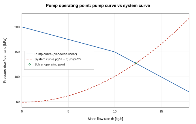
Figure 7. Pump operating point: pump curve, system curve, and the solver's converged operating point at their intersection.
Conclusions
The steady incompressible capability of OpenFLUME reproduces all six classical hydraulics benchmarks — laminar and turbulent single-pipe flow, parallel splits, multi-loop networks, hydrostatics, and pump/system operating points — to within 9.98e-10 %, the Newton convergence floor. Because every case was constructed as an exact closure of the solver's own friction laws (64/Re laminar, fixed-f Darcy–Weisbach, square-law resistance, piecewise-linear pump curve, ρgΔz elevation), the residual deviations measure the solver's algebraic convergence rather than any modeling gap; the Kirchhoff loop-closure sums of the multi-loop case confirm the same at the network level. Reynolds-correlation accuracy (Swamee–Jain vs Colebrook) is covered separately by the CI friction-factor tests and is deliberately excluded here by fixing f. Together with the compressible report, this establishes the solver's verification baseline across both incompressible and compressible steady regimes.
References
- White, F. M., Fluid Mechanics, 7th ed., McGraw-Hill, 2011.
- Cross, H., "Analysis of Flow in Networks of Conduits or Conductors," University of Illinois Engineering Experiment Station Bulletin No. 286, 1936.
- Streeter, V. L., and Wylie, E. B., Fluid Mechanics, 8th ed., McGraw-Hill, 1985.
- Swamee, P. K., and Jain, A. K., "Explicit Equations for Pipe-Flow Problems," Journal of the Hydraulics Division, ASCE, Vol. 102, No. 5, 1976, pp. 657–664.
- Majumdar, A. K., LeClair, A. C., Moore, R., and Schallhorn, P. A., Generalized Fluid System Simulation Program, Version 6.0, NASA/TM-2013-217492, 2013.
Nomenclature
| Symbol | Meaning |
|---|---|
| A | flow area |
| D | pipe diameter |
| f | Darcy friction factor |
| g | gravitational acceleration (9.80665 m/s²) |
| K | resistance loss coefficient |
| L | pipe length |
| ṁ | mass flow rate |
| P | static pressure |
| Q | volumetric flow rate |
| R | square-law resistance, ΔP = R·ṁ|ṁ| |
| Re | Reynolds number ρVD/μ |
| V | mean velocity |
| z / Δz | elevation / elevation change |
| ΔP | pressure difference |
| μ | dynamic viscosity |
| ρ | density |
| 0 | reference (bottom-of-column) property |