Tutorial: tank blowdown

Using Tank blowdown, the smallest shipped transient, you:

1. run it and read the time-history plots;
2. check it against the closed-form solution for adiabatic choked blowdown;
3. change it and find where that closed form stops applying;
4. sweep the orifice size.

Open "Tank blowdown" in the app →

What it models

A rigid 0.1 m³ tank of air vents to atmosphere through a sharp-edged orifice. The tank exchanges no heat with its surroundings, so the gas cools as it expands; that cooling is the main physics in this case.

The network has three elements:

• Tank: an internal fluid node whose volume turns on the mass and internal-energy storage terms, so P and T are integrated in time.
• Ambient: a boundary node, an infinite reservoir at fixed P and T.
• Orifice: the branch between them. For a gas it applies an expansibility factor and chokes when the pressure ratio drops below the critical value (manual §4.3.2).

Parameters

From tankBlowdown in src/ui/examples.ts:

Item	Field	Value
Solver	mode	transient, fixed step
	dt / endTime	0.01 s / 5.0 s
	tolerance, maxIterations, relaxation	1×10⁻⁶, 200, 0.9
Fluid	model	ideal gas, air preset (R = 287 J/(kg·K), γ = 1.4)
Tank	internal node	500 000 Pa, 300 K, volume 0.1 m³
Ambient	boundary node	101 325 Pa, 300 K
Orifice	orifice	area 1×10⁻⁴ m², Cd = 0.6

The air preset constants come from IdealGas.AIR in src/core/fluids/index.ts. Text view (manual §6.10) shows all of these values in one place as .fn text.

Run it

Click Run. The toolbar shows t = … s / 5 s · dt = 0.01 s during the run; at the end the status pill reads Converged with the accepted step count (the manual's screenshot shows 501).

Read the time histories

Open the Results tab. A plot is one x axis plus a list of channels, and a new plot starts empty.

1. Under or plot a whole set…, choose Node pressure: tank pressure falls from 500 kPa, and ambient stays flat at 101 325 Pa.
2. Click + Plot for a second plot tab, then choose Node & solid temperature. Tank temperature falls well below 300 K.
3. Add a third plot with Branch mass flow to see the vent flow decay.

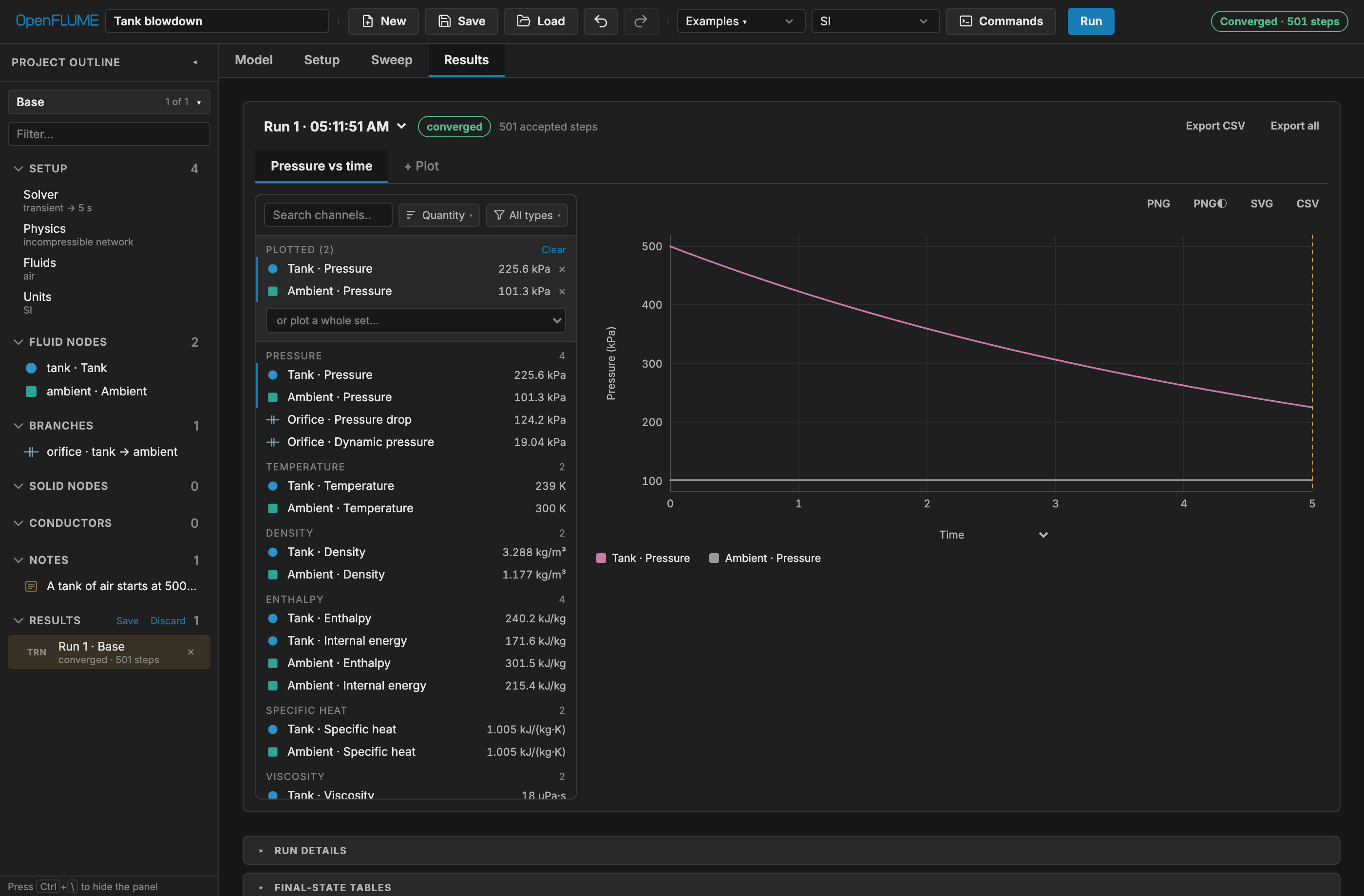
When reading these plots:

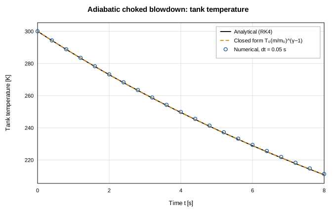
• The temperature drop is expected. The node stores internal energy (m·cv·T), while the outgoing flow carries enthalpy (cp·T). For an ideal gas in adiabatic blowdown this gives T/T₀ = (m/m₀)^(γ−1). A model that held the tank at 300 K throughout would have lost the flow-work term (manual §7.3).
• Ignore the branch flow at t = 0. That sample is the Newton warm start: the Initial flow guess, Auto (0.1 kg/s) unless you set one (manual §6.5). Read flows from the first step onward.
• Use the arrow keys on a focused chart to step the cursor between samples.
• Export CSV writes the plot's channels with time in the first column, plus provenance (model name, settings summary, config hash).
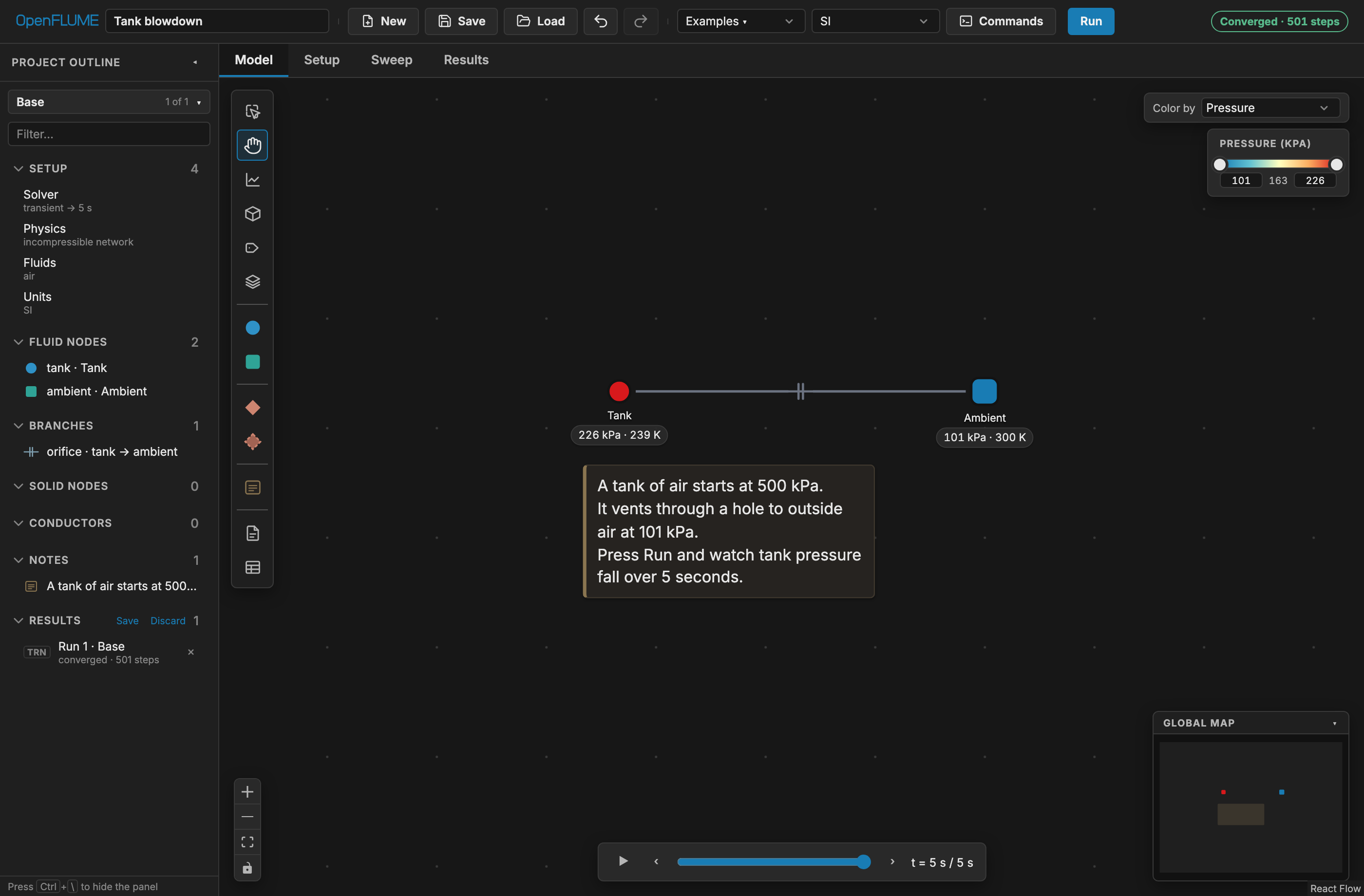
• On the Model tab, set Color by to Pressure and drag the time scrubber below the canvas to replay the run on the diagram.

Check it against the analytic solution

The transient tank validation report gives the closed form for adiabatic blowdown through a choked orifice. While the orifice stays choked:

m/m₀ = [1 + ((γ−1)/2) · t/τ]^(−2/(γ−1))
P/P₀ = (m/m₀)^γ
T/T₀ = (m/m₀)^(γ−1)

τ = V / ( Cd·A · √(γ R T₀) · (2/(γ+1))^((γ+1)/(2(γ−1))) )

The time constant τ depends on V, Cd·A, T₀ and the gas, but not on P₀. Case 1 of the report uses this example's V = 0.1 m³, Cd = 0.6, A = 10⁻⁴ m², and T₀ = 300 K and reports τ = 8.295 s; it starts from 10 bar instead of 5 bar, which leaves τ unchanged.

Choking. For γ = 1.4 the orifice chokes while P_ambient / P_tank ≤ 0.5283, that is, while the tank is above 101 325 / 0.5283 ≈ 191.8 kPa. The closed form reaches that pressure at t ≈ 6.1 s, so it applies to the whole 5 s run.

The closed form with the example's numbers (γ = 1.4, P₀ = 500 kPa, T₀ = 300 K, τ = 8.295 s) gives these reference values:

t [s]	P_tank, closed form [kPa]	T_tank, closed form [K]
1	423.2	286.0
2	359.6	273.0
3	306.7	260.9
4	262.5	249.5
5	225.4	238.9

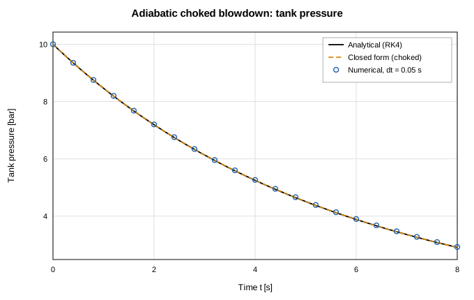
Compare these with tank pressure and temperature read from your plots. Expect the solver to sit slightly above the closed-form pressure: backward Euler evaluates the vent flow at the lower-pressure end-of-step state, so each step discharges slightly too little mass. The lag is one-sided and shrinks linearly with dt. In the report's time-step study the maximum pressure-trace deviation is 1.16 % of P₀ at dt = 0.4 s and 0.15 % at dt = 0.05 s, with an observed convergence order of 0.99–1.00. The example's dt = 0.01 s is five times finer than the finest step in that study.

For a scripted check, run the same model from Python (Python package):

import numpy as np
import openflume as of

res = of.example("Tank blowdown").solve()
t = np.asarray(res.times)
P = np.asarray(res.series("tank", "pressure"))

g, R, T0, V, CdA, P0 = 1.4, 287.0, 300.0, 0.1, 0.6e-4, 5e5
tau = V / (CdA * np.sqrt(g * R * T0) * (2 / (g + 1)) ** ((g + 1) / (2 * (g - 1))))
P_exact = P0 * (1 + (g - 1) / 2 * t / tau) ** (-2 * g / (g - 1))

print(f"tau = {tau:.3f} s")
print(f"max |P - P_exact| / P0 = {np.max(np.abs(P - P_exact)) / P0:.2e}")

The report also covers two-tank equalization, adiabatic fill heating, and blowdown through a scheduled valve. Its figures compare the solver with an RK4 reference and the closed form:

Modify it

Each change below is a single edit. After an edit, the existing result is marked stale until you run again (manual §8.7).

Run longer. In Setup → Solver, set End Time to 15 s and rerun. At about 6.1 s the orifice unchokes; the decay slows and the closed form no longer applies. Tank pressure approaches 101 325 Pa without overshooting.

Double the orifice area. Select the orifice branch and set its area to 2×10⁻⁴ m². τ halves to about 4.15 s. The tank now reaches the unchanged unchoking pressure (≈ 191.8 kPa) after roughly 3 s instead of 6 s, so the choked closed form no longer agrees over the subsonic remainder of the run.

Change the time step. Set Time Step to 0.1 s, then 0.2 s, and compare runs on one plot (see below). The deviation from the closed form should grow in proportion to dt, the first-order behavior the report measures. You can also try Adaptive stepping (manual §4.6.3).

Make the tank isothermal. Add an Ambient node at 300 K, drag from the tank to it, and choose a convection tie with h·A far above 10⁴ W/K; manual §3.6 says this holds the tank within about 1 K of the set point. Pressure then decays more slowly because the gas no longer cools as it expands, a useful control case against the adiabatic default.

Compare runs. Every run is kept in the run history. On any plot, + Compare run… overlays up to four recorded runs, dashed and interpolated onto the plot's axis, so runs with different time steps line up (manual §6.8).

Sweep the orifice size

The Sweep tab runs one parameter across up to 25 values (manual §6.9). Sweeps last only for the session and are never written to the model file.

1. Open Sweep. Under Define a sweep, pick the orifice branch's area as the Sweep target (the filter box helps with long lists).
2. Set Start = 0.5e-4, End = 2e-4, Variants = 4. Sweep values are always SI, whatever your display preset.
3. Click Run Sweep. Variants solve sequentially in the worker, and the variant table reports each value's status, convergence, peak |ṁ|, pressure and temperature ranges, and duration.
4. Export CSV writes the variant table. Promote on a row saves that variant as a named simulation variant with its run attached, to compare against the base run on one plot or save in the .fn file.

Each sweep job solves a frozen, hashed snapshot of the model. If you edit the model afterwards, the job shows a staleness banner.

Scope

This example is an ideal-gas, adiabatic, lumped tank with no wall heat capacity, real-gas effects, or stratification; the validation report lists wall heat transfer and real-fluid tank thermodynamics as out of scope. For a real-fluid tank with wall heat transfer, see the LH2 tank no-vent fill and Extension: Cryo tank vent control examples in the examples gallery.