Getting started

In about five minutes you run a steady case you can check by hand and a transient, then save your work. Local and Python installs are optional. The user's manual covers each step in depth, and its §2.3 (First Simulation) is this walkthrough in reference form.

OpenFLUME is alpha software (version 0.3.1), written by one engineer with heavy AI assistance. The project's position is check it rather than trust it, and the first two steps let you do that.

1. Open the app

Open openflume.github.io/OpenFLUME. No install or account is needed. The solver runs in a Web Worker in your browser, real-fluid properties come from CoolProp compiled to WebAssembly, and your model never leaves your machine.

The app opens with an empty canvas, or with the last model you had open (it autosaves to browser storage).

2. Run a case you can check by hand

Open the orifice sanity check directly:

Open "Sanity: orifice hand-calc" →

Or use the toolbar: Examples ▾ → Verify-by-inspection → Sanity: orifice hand-calc. Opening a link while the browser holds a model prompts before replacing it; loading from Examples ▾ replaces the current network without asking, so save any work you want to keep first.

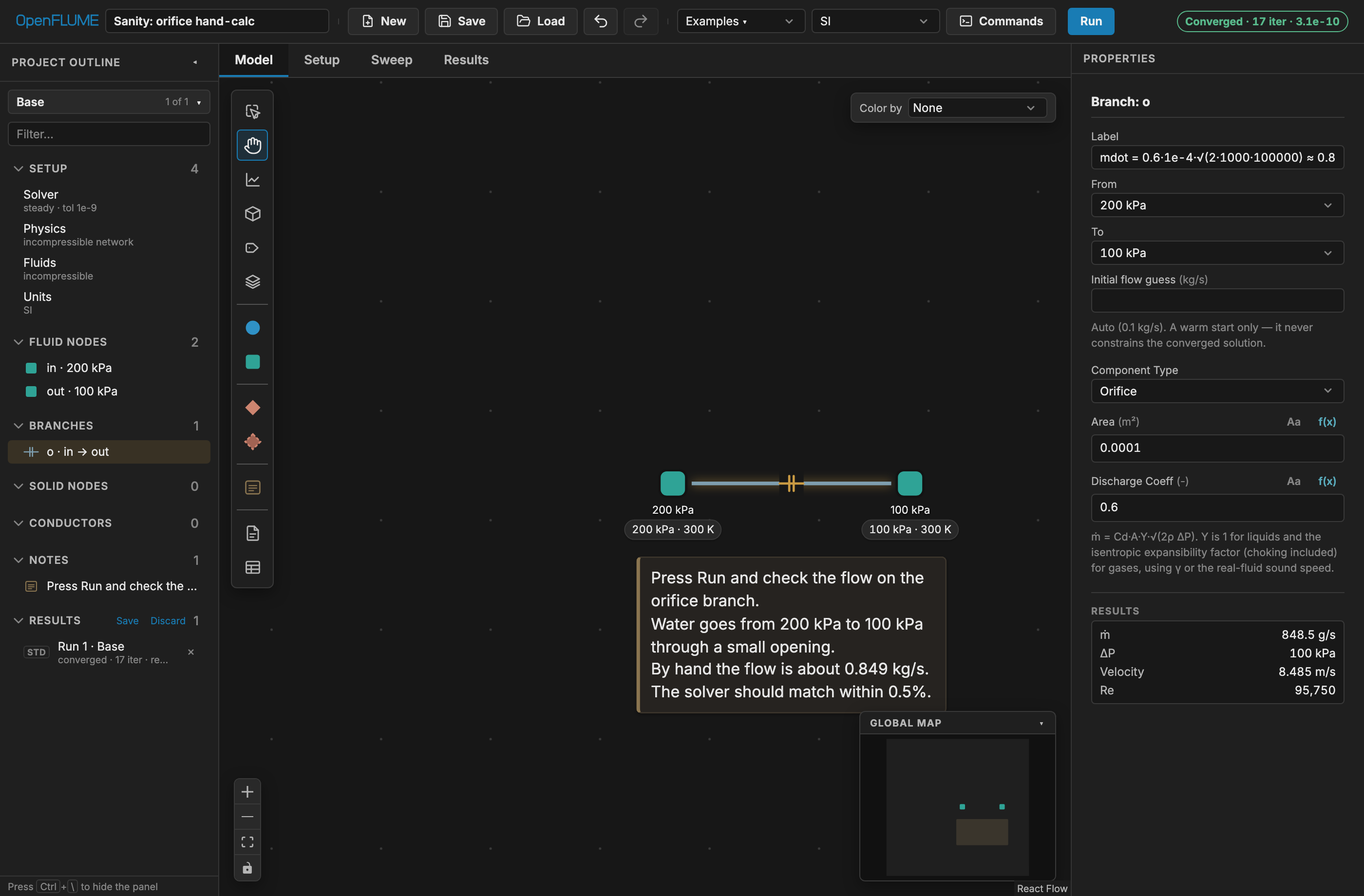
The model is two boundary nodes joined by one orifice branch:

Item	Value
Fluid	Incompressible, ρ = 1000 kg/m³, μ = 1×10⁻³ Pa·s, cp = 4182 J/(kg·K)
Upstream boundary	200 kPa, 300 K
Downstream boundary	100 kPa, 300 K
Orifice	area A = 1×10⁻⁴ m², discharge coefficient Cd = 0.6

The values come from sanityOrificeHandCalc in src/ui/examples.ts; a canvas note states the expected answer.

1. Click Run. The status pill at the right of the toolbar should read Converged, with an iteration count and final residual.
2. Click the orifice branch. Its solved mass flow appears in the Results block at the bottom of the property panel.

By hand, for an incompressible orifice:

ṁ = Cd · A · √(2 ρ ΔP)
  = 0.6 × 1e-4 × √(2 × 1000 × 100 000)
  = 0.6 × 1e-4 × 14 142
  ≈ 0.8485 kg/s

The manual (§7.1) requires the solver to match this within 0.5 %; its screenshot shows 848.5 g/s. Depending on your Units ▾ preset, the panel may show g/s, kg/h, or lbm/s; switch to SI to see kg/s.

This is the smallest case that exercises the whole chain (decode, validate, assemble, Newton solve, report). If it doesn't converge to the hand value, something is wrong with the installation or the code; please report it.

3. Run a transient: tank blowdown

Open "Tank blowdown" →

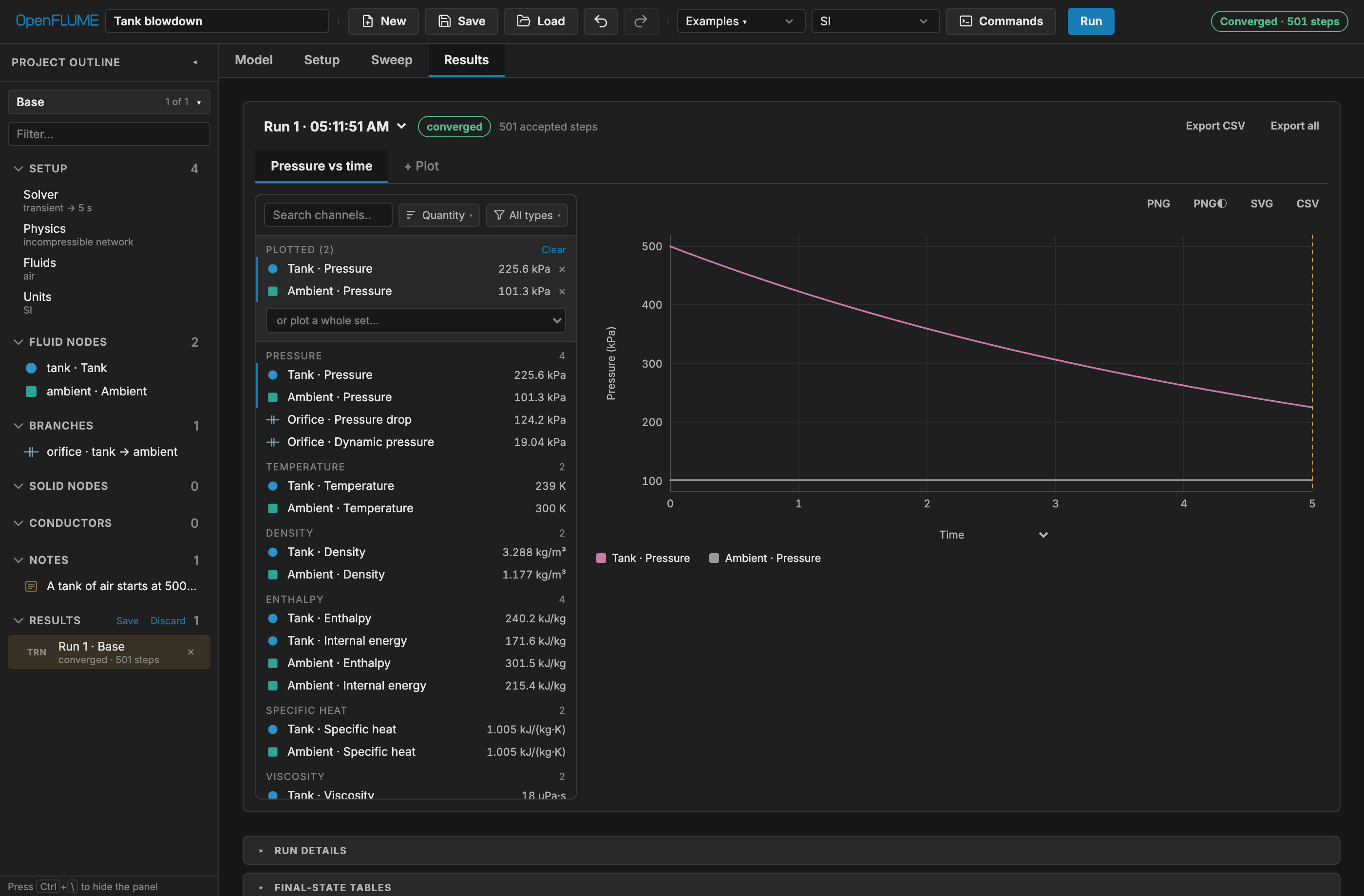
(Or Examples ▾ → Applications → Tank blowdown.) A 0.1 m³ tank of air at 500 kPa and 300 K vents through an orifice to 101 325 Pa for 5 s, with a fixed 0.01 s time step.

1. Click Run. The toolbar shows live t = … s / … s progress; at the end the status pill reports Converged with the number of accepted steps.
2. Open the Results tab. A new plot starts empty. Under or plot a whole set…, choose Node pressure. Tank pressure falls smoothly and monotonically from 500 kPa.
3. Choose Node & solid temperature. Tank temperature drops well below 300 K: the model captures adiabatic expansion cooling.
4. Back on the Model tab, a time scrubber now sits under the canvas. Set Color by to Pressure and drag it to replay the blowdown.

The tank blowdown tutorial checks this run against the closed-form choked-blowdown solution, then changes the orifice and runs a parameter sweep.

4. Save and load .fn files

• Save downloads the model as a .fn file: line-oriented text in SI units that you can diff and review (manual Appendix C). It holds the model and every variant but no results. If you have recorded runs, Save also writes a <model>.runs.json sidecar next to it.
• Load opens a .fn file or reattaches a .runs.json sidecar to the open model. A file that fails to parse never replaces the open model.
• If a file contains embedded JavaScript components, the app asks whether you trust that code before loading it. User code is trusted, not sandboxed, so accept it only from sources you trust.
• The browser autosaves the current model and run history, so a reload loses nothing. Autosave is not a backup; save a file for anything you want to keep.

5. Install locally (optional)

The hosted app and a local copy run the same code. Install locally to work offline, run the test suites, or keep user components on disk. You need Node.js 22 (pinned in .nvmrc) and npm 10.8 or newer:

git clone https://github.com/OpenFLUME/OpenFLUME.git
cd OpenFLUME
npm install
npm run dev        # http://localhost:5173

npm run serve builds the app and serves it with the optional companion server, which discovers user-component files under library/components (manual §2.4). OpenFLUME is not published to npm; to call the TypeScript core from your own scripts, import it from the source tree (manual §5.5).

6. Use it from Python (optional)

pip install openflume

The package bundles a Node.js runtime and runs the same src/core solver as the web app, so no JavaScript tooling is needed:

import openflume as of

net = of.example("Sanity: orifice hand-calc")
result = net.solve()
print(result.converged, result.branch("o")["mdot"])   # ≈ 0.8485 kg/s

net = of.load("my_model.fn")      # any model saved from the web app

See Python package for the full API, transient results as numpy/pandas, and parallel sweeps.

Where next

• Tank blowdown tutorial: verify a transient against a closed-form solution, then modify and sweep it.
• Build a propellant feed line: a LOX feed system from scratch with real-fluid properties.
• Cryogenic line chilldown: two-phase flow, film boiling, and conjugate heat transfer.
• Examples gallery: all 14 built-in models, each with a one-click link.
• Coming from GFSSP or SINDA/FLUINT: how the concepts map across.
• Before you rely on a result, read manual §1.7 (scope boundaries) and §8 (verification and validation). Known limits: no shock capture, no acoustic or water-hammer waves, two-phase flow by the homogeneous equilibrium model (HEM) only, and pump curves as the only turbomachinery model.