OpenFLUME, Version 0.3.1

Open FLUid Model Environment

User's Manual

John Rising

---

Document status: This manual covers OpenFLUME v0.3.1 and is maintained within the repository. In the event of a conflict between this documentation and the source code, src/core/schema.ts and src/core/validate.ts serve as the authoritative source of truth.

How to cite. See CITATION.cff, or:

Rising, J. (2026). OpenFLUME: Open FLUid Model Environment (v0.3.1). https://github.com/OpenFLUME/OpenFLUME

---

Preface

The aerospace industry has long needed an accessible, open-source tool for thermal-fluid network analysis. While legacy codes like NASA's GFSSP and C&R Technologies' SINDA/FLUINT are highly capable and validated, they can be difficult to extend, challenging to automate, and largely inaccessible to students, researchers, and engineers without institutional licenses. As a result, many organizations build their own proprietary network solvers—duplicating effort, repeating common mistakes, and re-running the same validation benchmarks without contributing to a shared foundation.

OpenFLUME aims to break this cycle. It solves this same class of problems using a proven finite-volume network formulation, provided entirely open-source.

Although a browser interface is provided, the solver core is a plain library with no user-interface dependency so it can be integrated into a research pipeline. The tool is designed to be easily understood and clear, so simulations can be created programmatically or, especially in the case of very large networks, AI-assisted.

This manual is organized so that a new user can stop after section 2 and still run a useful model. Section 1 introduces the method and limitations. Section 2 installs the program and walks through a first simulation. Sections 3 and 4 describe the data structure and the mathematical formulation. Section 5 covers program structure and scripting. Section 6 describes the interface. Section 7 describes example problems, and section 8 records verification and validation.

An engineer with an undergraduate background in fluid mechanics and heat transfer should be able to build a defensible model from this manual.

---

Executive Summary

OpenFLUME (Open FLUid Model Environment) is a finite-volume, general-purpose program for simulating arbitrary thermo-fluid networks, in both steady state and transient operation. The system under analysis is discretized into fluid nodes, branches, solid nodes, and conductors. Scalar properties like pressure, temperature, density, enthalpy, quality, and species composition are computed at nodes; mass flow rates are computed in branches and heat transfer rates in conductors.

The program runs entirely in a web browser. A visual network editor is backed by a solver that executes in a dedicated worker thread so that long runs do not block the interface. Models are saved as .fn text files and autosaved to browser storage. Everything runs locally, and nothing is transmitted to a server.

Four equation-of-state classes are supported: constant-density incompressible liquid, ideal gas with user-settable gas constants, thermal-expansion liquids (for buoyancy-driven circulation), and real fluid through a CoolProp WebAssembly sidecar. Seventeen branch component types model momentum sources and sinks: pipe, orifice, cavitating venturi, generic resistance, valve, check valve, dynamic check valve, relief valve, pump, bend, area change, flow source, pressure regulator, heated pipe, tabulated pressure drop, Reynolds-dependent custom resistance, and user-authored components. Conjugate heat transfer is available through solid lumped masses and ambient reservoirs linked by conduction, convection, and radiation conductors, with a temperature-dependent material catalogue and five convection heat-transfer models including two cryogenic chilldown correlations. CEA-coupled reacting junctions (steady or transient) support LOX/RP-1 and LOX/methane combustors, while the separate species-transport path supports transient ideal-gas chemistry.

The steady-state solver uses a coupled Newton–Raphson method to simultaneously resolve mass and momentum residuals. In challenging convergence scenarios, it leverages an analytic Jacobian (computed via forward-mode automatic differentiation), trust-region dogleg globalization, and pseudo-transient continuation. Transient simulations use a fully implicit backward-Euler scheme, supporting both fixed and variable time steps. Advanced optional capabilities include lumped fluid inertia, trapped-gas cushions, multi-species advection with stiff Arrhenius kinetics, declarative logic registers, transient PID control, and built-in parameter sweeps.

Thirteen example problems ship with the program, spanning hand-checkable sanity cases, engineering applications, and published benchmarks.

---

Nomenclature

Symbol	Quantity	Unit
$A$	flow or heat transfer area	m²
$a$	speed of sound	m/s
$C$	quadratic loss coefficient, $1/(2\rho C_d^2 A^2)$	1/(kg·m)
$C_d$	discharge coefficient	—
$d$	orifice or pipe bore (diameter ratio $\beta = d/D$)	m
$c$	damping coefficient (dynamic check valve)	N·s/m
$c_p$	specific heat at constant pressure	J/(kg·K)
$c_v$	specific heat at constant volume	J/(kg·K)
$D$	diameter (hydraulic)	m
$F$	radiation view factor; also force ($F_\text{preload}$)	—; N
$f$	Darcy friction factor	—
$G$	mass flux	kg/(m²·s)
$g$	gravitational acceleration, 9.80665	m/s²
$h$	specific enthalpy; also liquid height (hydrostatic-column check)	J/kg; m
$h_0$	stagnation enthalpy, $h + \tfrac12 v^2$	J/kg
$h_c$	convection heat transfer coefficient (property panel: Specified h)	W/(m²·K)
$\mathbf{J}$	Jacobian of the residual	—
$K$	loss coefficient, including $K_{90}$, $K_\text{bend}$, $K_\text{exp}$, $K_\text{con}$	—
$k$	thermal conductivity; also spring stiffness	W/(m·K); N/m
$L$	length	m
$M$	Mach number, $v/a$	—
$\dot m$	mass flow rate	kg/s
$m$	mass	kg
$\mathrm{Nu}$	Nusselt number	—
$n$	polytropic index	—
$O/F$	oxidizer-to-fuel mass ratio	—
$P$	pressure	Pa
$P_v$	saturation (vapor) pressure	Pa
$\mathrm{Pr}$	Prandtl number	—
$p$	valve or poppet fractional opening	—
$Q$	volumetric flow rate	m³/s
$\dot Q$	heat transfer rate	W
$R$	specific gas constant; also reverse-flow resistance $R(\dot m)$	J/(kg·K); Pa·s/kg
$\mathbf{R}$	residual vector	—
$\mathrm{Re}$	Reynolds number	—
$r$	pressure ratio $P_\text{down}/P_\text{up}$; also venturi recovery factor	—
$r_*$	critical (choke) pressure ratio, $(2/(\kappa+1))^{\kappa/(\kappa-1)}$	—
$T$	temperature	K
$T_0$	stagnation temperature; also EOS reference temperature	K
$t$	time	s
$UA$	overall conductance	W/K
$u$	specific internal energy	J/kg
$V$	volume	m³
$v$	velocity	m/s
$\mathbf{x}$	Newton unknown vector	—
$x$	vapor quality; also poppet travel	—; m
$Y$	ISO/AGA expansibility factor; also Miropolskii two-phase factor; also species mass fraction	—
$z$	elevation (positive up)	m
$\beta$	volumetric thermal expansion coefficient; also orifice diameter ratio ($d/D$)	1/K; —
$\gamma$	ratio of specific heats	—
$\Delta P$	pressure drop, $P_\text{from} - P_\text{to}$	Pa
$\Delta T$	temperature difference	K
$\Delta t$	time step	s
$\Delta z$	elevation change, $z_\text{to} - z_\text{from}$	m
$\varepsilon$	pipe roughness; also effectiveness; also emissivity	m; —; —
$\epsilon$	smoothing scale in $\tanh$ switches	kg/s
$\eta$	energy-release efficiency (reacting junction)	—
$\kappa$	isentropic exponent ($\gamma$ for an ideal gas; $a^2\rho/P$ for a real fluid)	—
$\mu$	dynamic viscosity	Pa·s
$\rho$	density	kg/m³
$\rho_0$	reference density (expandable-liquid EOS)	kg/m³
$\sigma$	Stefan–Boltzmann constant, 5.670374×10⁻⁸	W/(m²·K⁴)
$\tau$	time constant	s
$\theta$	bend angle	deg
$\omega$	under-relaxation factor	—

Subscripts. from, to — branch or conductor endpoints in declared orientation. up, down/dn — upstream, downstream by sign of $\dot m$. f, g — saturated liquid, saturated vapor; g is also the cushion gas volume $V_g$. w — wall; also the incompressible liquid volume $V_w$ in a cushion. sat — saturation. 0 — stagnation or EOS reference. src — source. c — component drop $\Delta P_c$, or chamber ($P_c$). disc, stroke, preload, crack, full — dynamic / relief-valve geometry and set-points. in, out — area-change ports. set — regulator set pressure. top — free surface of a hydrostatic column. arc — bend centreline arc.

Superscripts. $n$, $n+1$ — time level. $|\mathbf{R}|_\infty$ — infinity norm of the residual.

Abbreviations.

Abbreviation	Meaning
AD	Automatic differentiation
BDF1	First-order backward differentiation formula
CEA	Chemical Equilibrium with Applications
CFD	Computational fluid dynamics
DAE	Differential-algebraic equation
EOS	Equation of state
FD	Finite difference
HEM	Homogeneous equilibrium model
HEOS	Helmholtz Energy Equation of State
HEX	Heat exchanger
LHP	Loop heat pipe
NTU	Number of transfer units
ODE	Ordinary differential equation
P&ID	Piping and instrumentation diagram
PID	Proportional–integral–derivative
PTC	Pseudo-transient continuation
TVS	Thermodynamic vent system

---

Contents

1. Introduction
2. Installation and First Run
3. Data Structure
4. Mathematical Formulation
5. Program Structure
6. Graphical User Interface
7. Example Problems
8. Verification and Validation
9. Appendix A — Branch Component Quick Reference
10. Appendix B — Conductor Quick Reference
11. Appendix C — The .fn File Format
12. Appendix D — Glossary
13. Appendix E — References

---

1. Introduction

1.1 Purpose and Scope

This program computes the distribution of pressure, temperature, density, and mass flow rate in a network of pipes and components, together with the temperature distribution in solid structure thermally coupled to that fluid. It addresses the class of problem in which the system behavior is the question — how much flow each leg of a manifold takes, how fast a tank blows down, how hot a cooling channel wall runs, when a cryogenic line finishes chilling — as distinct from problems in which the local flow field inside a single component is the question, which require computational fluid dynamics.

Typical applications include propellant feed and pressurization systems, vent and relief circuits, regenerative cooling jackets, water and process distribution networks, cryogenic transfer lines, passive-circulation loops, and spacecraft thermal control loops.

1.2 Network Flow Analysis

The system is represented as a directed graph. Control volumes are placed at nodes, where the extensive fluid state is stored and conservation of mass and energy is enforced. Branches connect pairs of nodes, and each branch carries one scalar unknown, its mass flow rate, governed by a momentum relation between the pressures at its two endpoint nodes.

You might wonder why the program separates nodes (volume) and branches (flow) instead of just offering a single "pipe" component that has both. This staggered approach is standard in thermal-fluid network solvers because it handles complex junctions naturally: a single node can connect to any number of branches without needing to define which pipe "owns" the junction's volume. It also avoids numerical instabilities that often occur when mass and momentum are computed at the exact same location.

Figure 1-1. A representative network: two pressure boundaries, six internal nodes, and twelve branches forming interconnected loops. This topology is the multi-loop verification case of docs/validation/incompressible-hydraulics-report.md.

Two consequences of this arrangement dictate how you will build and scope your models:

First, spatial resolution is entirely up to you. A 100 m pipe represented by a single branch has only one flow rate and no interior temperature profile. If you represent that same pipe with twenty branches and nineteen interior nodes, you can capture an axial temperature profile and a distributed friction gradient. Wherever a gradient matters to your result you must subdivide the line into enough segments to resolve it. (The shipped chilldown example uses twenty axial segments for a 61 m line for exactly this reason; the Repeat and Split commands of section 3.13 build such discretizations.)

Second, a node's volume determines its ability to store mass and energy. In a steady-state run, volume is irrelevant and you can safely ignore it. In a transient run, however, an interior node accumulates mass and energy in proportion to its volume. This means you must assign a positive volume to every interior node in a transient model, because how you distribute that volume directly sets your system's behavior.

1.2.1 Network Definitions

Fluid node. A control volume holding fluid state. An internal (interior) node has unknown pressure and temperature solved by the program. A boundary node has its pressure and temperature imposed, either as constants or from a time schedule; it acts as an infinite reservoir. Every network must contain at least one boundary node, which anchors the pressure level of the whole system.

Branch. A directed connection between two fluid nodes carrying a mass flow rate. Its component assigns the momentum relation — pipe friction, an orifice closure, a pump curve, and so on. Both endpoints must be fluid nodes resolving to the same named fluid, and a branch may not connect a node to itself.

Solid node. A lumped thermal mass with a temperature, a mass, and a specific heat. It holds no fluid and passes no flow.

Ambient node. A fixed-temperature thermal reservoir of effectively infinite capacity, optionally driven by a temperature schedule. It plays the same role in the thermal network that a boundary node plays in the fluid network.

Conductor. A directed thermal link carrying a heat transfer rate by conduction, convection, or radiation. Conduction and radiation conductors join two thermal (solid or ambient) nodes. A convection conductor is the fluid-solid coupling: exactly one endpoint must be a fluid node and the other a solid or ambient node.

Group (subnetwork). A purely visual container for organizing a large diagram. The solver ignores groups; a grouped network produces identical numbers to an ungrouped one.

Note. A free-floating text annotation. Notes are inert — the solver never reads them and they are excluded from the provenance hash, so documenting a model never invalidates its results.

1.3 Units

All quantities in a model are SI. The solver, the saved .fn file, and the scripting interface use SI exclusively and carry no unit metadata.

Quantity	Unit	Quantity	Unit
Pressure	Pa	Volume	m³
Temperature	K	Mass	kg
Mass flow rate	kg/s	Heat rate, power	W
Density	kg/m³	Specific heat	J/(kg·K)
Dynamic viscosity	Pa·s	Thermal conductivity	W/(m·K)
Length, diameter, roughness	m	Heat transfer coefficient	W/(m²·K)
Area	m²	Overall conductance $UA$	W/K
Time	s	Activation energy	J/mol
Elevation	m (positive up)	Molecular weight	kg/mol

The interface can display and accept other units. The Units ▾ menu offers three presets — SI, Metric engineering, and US customary — which convert values in property fields for display and entry only, including degrees Rankine, °F, and psi. Conversion happens at the input and output; the stored model is always SI. Values typed into the parameter sweep workspace and into the model text editor are SI regardless of the display preset.

1.4 Sign Conventions

Sign errors are the most common cause of a physically wrong but numerically converged model. The four conventions below are enforced consistently throughout.

Mass flow. A branch is declared from one node to another. Positive mass flow is in the declared from → to direction. A negative reported $\dot m$ means the fluid runs backward through that branch relative to how you drew it, which is normal and correct for legs whose direction you did not know in advance.

Pressure drop. $\Delta P \equiv P_\text{from} - P_\text{to}$. A component's pressure-drop relation returns a positive value for a loss. A pump therefore returns a negative pressure drop, being a pressure rise in the from → to direction.

Elevation. elevationChange on a pipe is $z_\text{to} - z_\text{from}$, in metres, positive when the to end is higher. The hydrostatic contribution is $\Delta P_\text{elev} = \rho g\Delta z$ with $g = 9.80665$ m/s², so lifting fluid costs pressure. Elevation may instead be derived from physical node coordinates (section 3.10). Note that settings.gravity exists in the schema as a vector but hydrostatics currently use the fixed scalar $g$ above.

Heat. A conductor's heat rate is positive when heat flows from its from endpoint toward its to endpoint. A heatInput on any node, fluid or solid, is positive when heat is added to that node. In a fluid node's energy balance, convective heat arriving from a wall is positive.

1.5 Capability Summary

Category	Available
Solution modes	Steady state; transient with fixed or adaptive time step
Equations of state	Incompressible liquid, ideal gas, thermal-expansion liquid, real fluid (CoolProp, 124-fluid catalogue)
Two-phase	Transient homogeneous-equilibrium model for real fluids
Compressible duct flow	Opt-in quasi-1-D (momentumFlux + kineticEnergy, any fluid model): Fanno/Rayleigh choking, seeded supersonic nozzles
Branch components	17 types (Appendix A)
Conjugate heat transfer	Solid and ambient nodes; conduction, convection, radiation conductors
Convection models	Specified $h$ or expression, Dittus–Boelter, Miropolskii, Darr–Hartwig, TT-WF
Solid properties	Constant, sourced material catalogue, table, equation, time table
Transient momentum	Optional lumped fluid inertia; trapped-gas cushions
Species	Multi-species advective transport with Arrhenius chemistry (transient, ideal gas)
Combustion	CEA-coupled reacting junctions (steady or transient + kineticEnergy; LOX/RP-1 and LOX/CH₄)
Control and logic	Registers, declarative logic rules, stop rules, transient PID controllers
Multi-fluid	Named isolated fluid continua, mixed EOS classes allowed (wall-coupled only)
Extensibility	Tabulated $\Delta P$, $K(\mathrm{Re})$ resistances, user-authored JavaScript components
Exploration	Session-only single-parameter sweeps up to 25 variants
Persistence	.fn text save/load, browser autosave, 13 shipped examples

1.6 Program Structure

The program has four parts. The core (src/core) is a platform-agnostic TypeScript library containing the schema, validation, equations of state, component relations, and both solvers; it has no browser dependency and runs unchanged in Node.js. The substrate (src/substrate) implements the .fn text projection. The interface (src/ui) is a React application that owns the canvas, panels, run history, and a solver worker that keeps long solves off the main thread. An optional companion server (scripts/serve.ts) serves the built application and discovers user-authored component files on disk. Real-fluid properties come from a lazily loaded CoolProp WebAssembly module. Section 5 develops this in detail.

1.7 Scope Boundaries

The following limitations are structural. They follow from the lumped-parameter formulation and cannot be worked around by refining the mesh or tightening tolerances. Read this list before using a result to support a decision.

No shocks. With settings.momentumFlux and settings.kineticEnergy both enabled, the solver handles quasi-1-D compressible duct flow, specficially Fanno friction choking, Rayleigh thermal choking, and converging–diverging nozzles built from tapered pipe. Smoothly expanding supersonic branches are reachable, like converging-diverging nozzles. Under the default limited-upwind momentum faces (settings.momentumFluxScheme: "upwind", section 4.1.2) the transonic solve is seed-robust: entropy-violating roots such as a station dipping onto the supersonic branch mid-convergent do not satisfy the discrete equations at all, so even a flat cold start converges to the physical branch. The legacy "central" scheme is a couple of percent more accurate at the choke but must be seeded onto the physical branch (initialMdot near the choked value and a monotonically falling nodal $P$/$T$ guess); its converged root is certified by the second-law audit (settings.transonicAdmissibility).

What remains structurally out of scope is shock capture. There is no Rankine–Hugoniot jump condition and no mechanism for locating a normal shock, so over-expanded and separated nozzle operation, shock position, and any case where the flow must pass supersonic → subsonic cannot be modeled. Thrust is likewise not computed; the solver returns the internal flow field, not a momentum balance on the vehicle. Point choking at restrictions is separately available through orifice (expansibility $Y(r,\kappa)$, any gas-capable fluid) and cavitatingVenturi (choked liquid). With the flags off (the default), branch momentum is the incompressible algebraic relation $\Delta P(\dot m)$ with no Mach number in the formulation, and a long gas line driven toward sonic velocity returns unphysical answers rather than friction-choking.

Kinetic energy transport is opt-in and steady-oriented. By default static enthalpy is fluxed; the $\tfrac12 v^2$ term is not carried, so there is no stagnation/static distinction and recovery temperature and diffuser heating are not modeled. settings.kineticEnergy switches the energy equation to stagnation-enthalpy transport for any fluid model — the solver couples pressure, mass flow, and enthalpy in one Newton system ([P, ṁ, h]), which is what lets it hold near-sonic states, and enthalpy is a complete state coordinate for every EOS including CoolProp real fluids. The coupled system is not steady-only: transient solves take it too, for real fluids and for every analytic kineticEnergy network. Only species-transport networks keep the segregated stagnation-enthalpy update, composition not being a coupled unknown, and that path is not designed to track choking fronts.

No acoustic wave propagation. Optional lumped fluid inertia $(L/A)d\dot m/dt$ captures bulk surge, but there is no distributed wave equation or method-of-characteristics solution. Classical water hammer — wave timing, reflection, anything limited by the speed of sound — cannot be simulated.

Cavitation only at the venturi closure. There is no general cavitation-inception check on pumps, valves, or low-pressure liquid nodes.

Turbomachinery is a pump curve. Pressure rise versus volumetric flow only. No compressor or turbine maps, and no shaft-work term in the energy equation, so pump heating of the fluid is not captured.

No general junction mixing. Outside an explicitly declared reacting junction, unlike fluids may not meet at a node; couple them thermally through a solid wall instead. A reacting junction is the narrow exception: declared oxidizer and fuel inlet branches terminate at a chamber node and produce one named ideal-gas stream under the CEA closure. Different EOS classes may otherwise coexist in one network (e.g. an ideal-gas hot side with a real-fluid coolant) precisely because the wall is the only coupling — property access dispatches per node.

Two-phase flow is homogeneous-equilibrium. The HEM assumption suits dispersed, high-mixing, or low-quality flows. At high void fraction it under-predicts pressure drop relative to separated-flow correlations such as Lockhart–Martinelli, which are not implemented.

Reacting-flow support is split between two models. Species transport with Arrhenius chemistry is transient-only and ideal-gas-only. CEA-coupled reacting junctions are steady-only, require kineticEnergy, freeze product composition downstream, and support only the committed LOX/RP-1 and LOX/CH₄ tables though more can be generated by the user; see combustion.md.

User code is trusted, not sandboxed. Embedded and local components execute JavaScript through new Function. This is not a security boundary; treat component files like source code.

Steady closed ideal-gas loops need a pressure anchor. In a steady-state simulation, the solver finds a balance of flows. If a section of your network is completely sealed off (like a closed loop or a trapped section behind a closed valve), there is no fixed pressure boundary to tell the solver what the overall pressure inside that isolated section should be. For an ideal gas, this missing information makes the math unsolvable (a singular Jacobian). To fix this, connect a boundary node to the isolated section or run the model in transient mode (where the known initial pressure anchors the system over time).

1.8 How to Read This Manual

As a new user, you should first read section 1.4 (sign conventions), work through section 2, and then jump straight to the example in section 7 that most closely matches your problem so you can start modifying it. Sections 3 and 4 provide deep reference material—they are best read after you've built your first model and want to understand exactly what is happening under the hood. If you are preparing to publish a paper or certify an engineering result, you must read section 1.7 (limitations) and section 8 (verification) in full to ensure you are operating within the solver's validated bounds.

---

2. Installation and First Run

2.1 Prerequisites

Node.js 22 (the pinned version is in .nvmrc) and npm 10.8 or newer. A current Chromium-, Firefox-, or WebKit-based browser. No other services, licenses, or network access are required; real-fluid support is bundled, not fetched at run time.

2.2 Installation

git clone https://github.com/OpenFLUME/OpenFLUME.git
cd OpenFLUME
npm install
npm run dev

Open http://localhost:5173. The application loads with an empty canvas, or with your most recent network restored from browser storage.

2.3 First Simulation

The fastest way to confirm a working installation is to run a case whose answer is known in closed form.

1. Open Examples ▾ in the toolbar and choose, under Verify-by-inspection, Sanity: orifice hand-calc. Two boundary nodes appear, joined by a single orifice branch, with the expected answer written on the canvas as a note.
2. Click Run. The status pill reports Converged with an iteration count and final residual.
3. Select the orifice branch. The Results block at the bottom of the property panel shows the solved mass flow rate. It should agree with $C_d A\sqrt{2\rho\Delta P} \approx 0.8485$ kg/s to within 0.5 %.

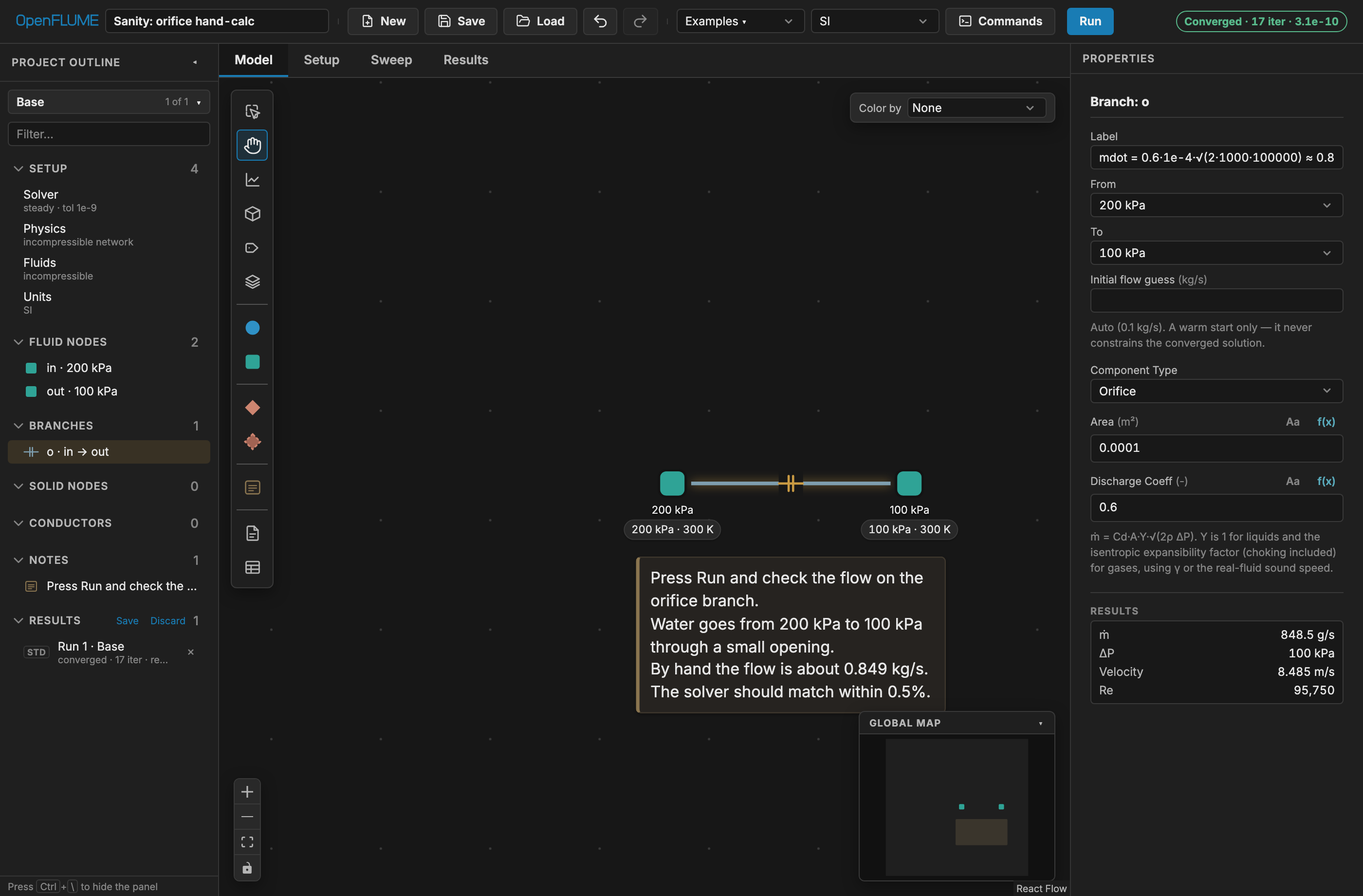
Figure 2-1. The orifice sanity check after a converged run. The status pill (top right) reports the iteration count and final residual; the property panel's Results block reports the solved mass flow of 848.5 g/s against the hand-calculated 0.849 kg/s.

Then run a transient:

1. Choose Tank blowdown from Applications — a 0.1 m³ air tank at 500 kPa, 300 K venting through an orifice to atmosphere over 5 s.
2. Click Run. The status pill reports Converged with the accepted step count. Open the Results tab. A new plot starts empty — from or plot a whole set… choose Node pressure to chart tank and ambient pressure versus time. Tank pressure should decay monotonically toward 101 325 Pa. The Node & solid temperature preset shows tank temperature falling well below its initial 300 K: the expansion is adiabatic, not isothermal.
3. Return to the Model tab. A time scrubber has appeared below the canvas; drag it and, with Color by set to Pressure, watch the network recolor through the blowdown.

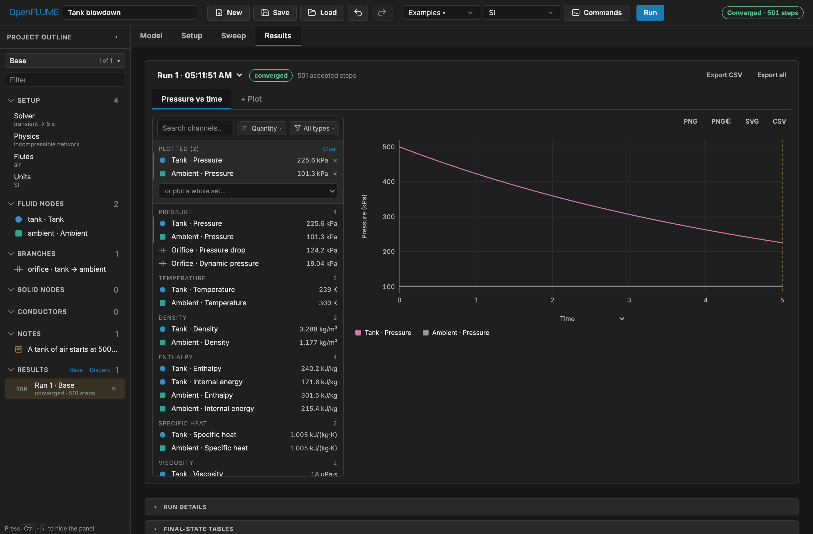
Figure 2-2. The Results tab after the tank-blowdown transient, with the Node pressure preset: tank pressure decays from 500 kPa toward atmosphere over the 5 s run, 501 accepted steps.

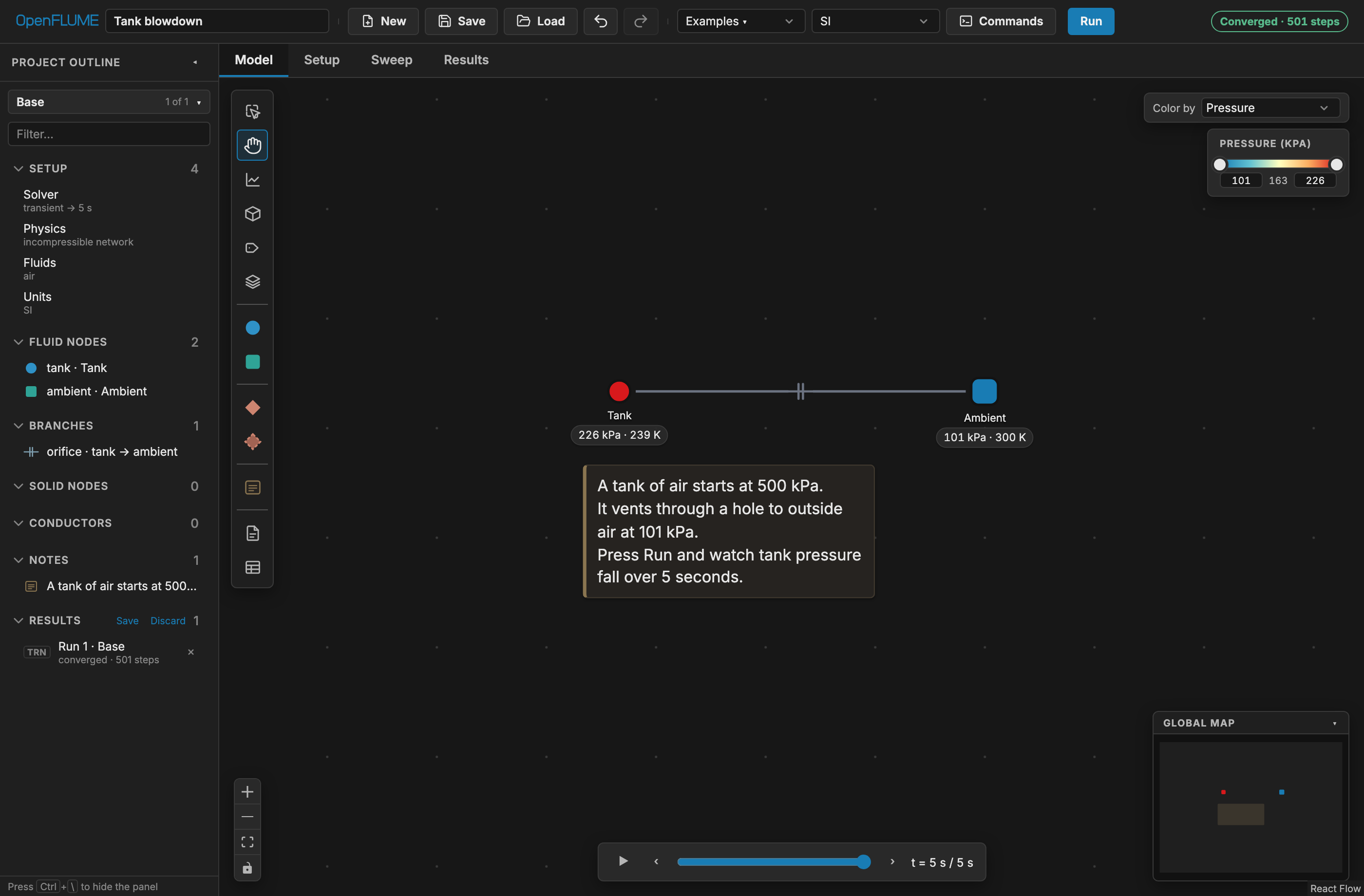
Figure 2-3. Back on the Model tab with Color by set to Pressure: the colormap legend appears at the top right and the time scrubber below the canvas replays the run.

If both cases converge, the installation is sound.

2.4 Companion Server (Optional)

The companion server is needed only for user-authored component files (section 5.6). It serves the built application and exposes the component library on the same origin:

npm run serve        # build, then serve on http://localhost:4174
npm run serve:dist   # serve an existing dist/ without rebuilding

Relevant environment variables are PORT, HOST, DIST_DIR, LIBRARY_DIR (default library/components), and ALLOW_REMOTE_WRITES. Component creation over HTTP is restricted to localhost and refuses to overwrite existing files.

2.5 Files Read and Written

Artifact	Direction	Notes
.fn model file	Save / Load	Line-oriented lossless text projection (Appendix C)
Browser localStorage	Autosave	Last network, unit preferences, and the session's run history; restored on reload
library/components/*.component.js	Read (and optional create)	User components; requires companion server
CSV exports	Write	Channel data, result tables, transient time series, sweep variants, run comparisons
Solver diary JSON / text	Write	Convergence record with config-hash provenance

2.6 Running the Test Suites

npm test          # fast pull-request tier
npm run check     # production build plus fast tier
npm run test:all  # every Vitest file
npm run test:slow # adds opt-in slow scientific validation blocks
npm run test:e2e  # builds and runs the Playwright end-to-end suite

Tiers are described in docs/testing-slow.md and section 8.5.

---

3. Data Structure

A complete model is a single NetworkConfig object. This section describes each element and its properties. Exact TypeScript declarations live in src/core/schema.ts; the constraints quoted here are enforced by src/core/validate.ts before any solve.

3.0 A Complete Model

Before the field-by-field reference, it is worth seeing the whole object at once. The listing below is the shipped Three-pipe junction example (section 7.2) in full — a steady incompressible case with one inlet boundary, one junction node, one outlet boundary, and two pipe branches. Every structure the rest of section 3 documents appears here in its concrete form: meta, settings, fluid, nodes, and branches.

{
  "meta": {
    "name": "Three-pipe junction",
    "version": 2
  },
  "settings": {
    "mode": "steady",
    "tolerance": 1e-9,
    "maxIterations": 500,
    "relaxation": 0.9
  },
  "fluid": {
    "model": "incompressible",
    "preset": "water"
  },
  "nodes": [
    {
      "id": "in",
      "type": "boundary",
      "x": 0,
      "y": 0,
      "pressure": 300000,
      "temperature": 300,
      "label": "Inlet"
    },
    {
      "id": "j",
      "type": "internal",
      "x": 200,
      "y": 0,
      "pressure": 250000,
      "temperature": 300,
      "label": "Junction",
      "volume": 0.001
    },
    {
      "id": "out1",
      "type": "boundary",
      "x": 400,
      "y": 100,
      "pressure": 200000,
      "temperature": 300,
      "label": "Out 1"
    }
  ],
  "branches": [
    {
      "id": "b1",
      "from": "in",
      "to": "j",
      "label": "Pipe 1",
      "component": {
        "type": "pipe",
        "length": 2,
        "diameter": 0.03,
        "roughness": 1e-5,
        "elevationChange": 0
      }
    },
    {
      "id": "b2",
      "from": "j",
      "to": "out1",
      "label": "Pipe 2",
      "component": {
        "type": "pipe",
        "length": 3,
        "diameter": 0.02,
        "roughness": 1e-5
      }
    }
  ]
}

Note what is absent. x and y are diagram pixels and never reach the solver. volume on the junction node is carried even though this is a steady case, where it is ignored — it costs nothing and makes the model runnable as a transient. elevationChange is stated explicitly on the first pipe and omitted on the second, which is the same thing: an omitted optional field takes its default rather than being an error. solidNodes, conductors, groups, and notes are all optional and simply do not appear.

The .fn file format is a line-oriented projection of exactly this object, not a different model; see Appendix C.

3.1 Top-Level Structure

Key	Required	Contents
meta	yes	name and version (must be 2)
settings	yes	Mode, tolerances, time stepping, solver strategy (section 3.11)
fluid	yes	Default equation of state for the network
fluids	no	Named additional fluids as isolated continua
nodes	yes	Fluid nodes, at least one, at least one of them a boundary
branches	yes	Fluid branches, at least one
solidNodes	no	Solid lumped masses and ambient reservoirs
conductors	no	Thermal links
species	no	Species list and Arrhenius reactions (ideal gas, transient)
junctions	no	CEA-coupled reacting junctions (steady or transient)
registers	no	Named numeric state for logic and expressions
logic	no	Declarative event rules and stop rules
controllers	no	Transient PID controllers
componentLibrary	no	Embedded user-component source
closureParams	no	Overrides for correlation constants
groups	no	Visual subnetwork containers
notes	no	Text annotations (inert)

Only schema version 2 is accepted. Decoding rejects unknown structure before validation runs, and validation runs before every solve.

3.2 Fluid Node Properties

Field	Type	Unit	Required	Meaning
id	string	—	yes	Unique; shares one namespace with solid nodes
label	string	—	no	Display name
type	internal / boundary	—	yes	Interior control volume or reservoir
x, y	number	px	yes	Diagram position; never a solver input
position	{x,y,z}	m	no	Physical coordinates, $z$ up; formula-bindable
group	string	—	no	Subnetwork membership
fluid	string	—	no	Names an entry in fluids; omit for the default
pressure	number	Pa	see below	Boundary value, or transient initial value
temperature	number	K	see below	Boundary value, or transient initial value
quality	number	—	alternative to temperature	Real fluid only; mutually exclusive with temperature
volume	number or expression	m³	internal, transient	Storage volume; must be positive
heatInput	number	W	no	Heat added to the node
pressureSchedule	[[t,P],…]	s, Pa	no	Boundary only
temperatureSchedule	[[t,T],…]	s, K	no	Boundary only
gasCushion	object	m³, —	no	Trapped gas; transient liquid networks only
massFractions	map	—	no	Species composition
fluidFrontInlet	number on [0,1]	—	no	Boundary only; cryogenic front inlet
initiallyWet	boolean	—	no	Capillary networks: liquid present at $t=0$ (§4.3.19)

A boundary node requires pressure, and either temperature or quality but not both. quality is accepted only when that node's fluid model is realFluid.

An internal node in a transient requires a positive volume, plus pressure and either temperature or quality as the initial condition. In steady state, an internal node needs neither: its pressure and temperature are unknowns, and any values supplied serve only as the starting iterate. Supplying a good initial guess is nevertheless the single most effective way to help a difficult steady case converge.

Note the distinction between x, y — pixel coordinates that place the symbol on the diagram — and position — physical coordinates in metres that can feed physics, notably derived pipe elevation change and derived convection axial stations.

3.3 Branch Properties

Every branch carries id, an optional label, from, to, and a component object whose type selects the momentum relation. Both endpoints must be fluid nodes, must resolve to the same named fluid, and must differ from each other.

The nineteen component types are pipe, orifice, cavitatingVenturi, resistance, valve, checkValve, dynamicCheckValve, reliefValve, pump, bend, areaChange, flowSource, regulator, heatedPipe, dpTable, customResistance, rectChannel, capillaryChannel, and userComponent. Their parameters, constraints, interface labels, and governing equations are tabulated in Appendix A and derived in section 4.3.

3.4 Solid Node Properties

Field	Type	Unit	Required	Meaning
id	string	—	yes	Unique across fluid and solid nodes
label	string	—	no	Display name
type	solid / ambient	—	yes	Lumped mass or fixed reservoir
x, y	number	px	yes	Diagram position
position	{x,y,z}	m	no	Physical coordinates
temperature	number	K	yes	Fixed value (ambient) or initial value (solid)
mass	number	kg	solid, transient	Lumped mass; must be positive
cp	number or spec	J/(kg·K)	solid, transient	Specific heat; see below
heatInput	number	W	no	Heat added to the node
temperatureSchedule	[[t,T],…]	s, K	no	Ambient only

A solid node has finite thermal capacity $m c_p$ and therefore a thermal time constant; in steady state its temperature floats to satisfy its heat balance and neither mass nor cp is required. An ambient node is a fixed-temperature reservoir of unbounded capacity, appropriate for a room, deep space, or a temperature-controlled bath.

cp accepts five forms: a constant; { material } naming an entry in the sourced catalogue (OFHC copper, GRCop-84, Aluminum 6061-T6, stainless 304 and 316, Inconel 718, PTFE, anisotropic G-10 CR — each with a documented validity range and end-value clamping); { table } of temperature–value pairs; { expression, tRange }; or { timeTable }, which is transient-only. Catalogue sources and validity ranges are recorded in docs/solid-properties-results.md.

3.5 Conductor Properties

Every conductor carries id, an optional label, from, to, and a type object discriminated by kind.

kind	Endpoints	Parameters
conduction	both thermal (solid or ambient)	k (W/(m·K), constant, spec object, or expression), area (m²), length (m)
convection	exactly one fluid, one thermal	area (m²), and either h (W/(m²·K)) or a correlation block
radiation	both thermal	emissivity, area (m²), viewFactor

The convection conductor is the only fluid-to-solid coupling in the program, and it is coupled implicitly: the fluid node's energy residual and the solid node's energy residual both carry the same conductor heat rate with opposite signs.

A correlation block replaces a constant $h$ with one computed from the local flow state. Its model is dittusBoelter, miropolskii, darrHartwig (which also needs axialPosition), ttWf (which also needs axialPosition and segmentLength, and is transient-only), or custom (which needs an expression). diameter must be positive; flowArea defaults to $\pi D^2/4$. All named models require the realFluid fluid model; custom does not. When a correlation is present, h becomes optional and a floor of 5 W/(m²·K) prevents zero conductance. Correlation forms are given in section 4.4.

A worked conjugate fragment: a heated wall lump tied to a fluid node by convection and to deep-space-like surroundings by radiation. Added to a network that already declares a fluid node fluid1, these two arrays are the whole thermal side of the model.

{
  "solidNodes": [
    {
      "id": "wall",
      "type": "solid",
      "x": 200,
      "y": 150,
      "temperature": 350,
      "mass": 1,
      "cp": 500,
      "heatInput": 5000
    },
    { "id": "amb", "type": "ambient", "x": 300, "y": 0, "temperature": 300 }
  ],
  "conductors": [
    {
      "id": "c1",
      "from": "wall",
      "to": "fluid1",
      "type": { "kind": "convection", "h": 1000, "area": 0.1 }
    },
    {
      "id": "c2",
      "from": "wall",
      "to": "amb",
      "type": {
        "kind": "radiation",
        "emissivity": 0.8,
        "area": 0.5,
        "viewFactor": 1
      }
    }
  ]
}

The wall node carries mass and cp because it is a lumped capacity; amb carries neither, being a reservoir. Conductor c1 has exactly one fluid endpoint, which is what makes it legal as a convection tie, and its heat rate appears with opposite signs in the wall and fluid1 energy residuals.

3.6 Ambient Nodes and Boundary Thermal Conditions

To impose a wall temperature, connect the wall solid node to an ambient node through a conductor sized for the physics you intend: a large-conductance conduction or convection tie clamps the wall near the ambient temperature, while a radiation tie to a 4 K ambient represents deep space. The same trick makes a gas tank near-isothermal — attach a convection conductor with $hA \gg 10^4$ W/K between the tank fluid node and an ambient node, and the tank will track the set point within about 1 K, which is a useful control case against the adiabatic default.

3.7 Schedules

A schedule is an array of [time, value] pairs with time in seconds and the value in SI units for its quantity. Interpolation between knots is piecewise linear, and values outside the range clamp to the first or last entry. Available schedules are boundary node pressureSchedule and temperatureSchedule, ambient node temperatureSchedule, valve positionSchedule, and flow source massFlowSchedule.

Under adaptive time stepping, the step size is truncated so that every accepted step lands exactly on schedule breakpoints, which prevents a discontinuity from being straddled and smeared.

3.8 Registers, Logic, and Controllers

registers are named numbers that persist across a transient and are returned with the results. logic rules fire on lifecycle events, evaluate a guarded condition, atomically assign registers, and can stop the run with a stated reason — enough to build hysteresis bands, latches, event counters, and termination criteria without writing code. controllers are PID controllers that run on accepted transient steps and actuate valves, flow sources, boundary conditions, or heat inputs on the following step.

Controllers are transient-only, have no anti-windup, and take effect on the step after the one that measured the error unless initialOutput seeds the first step. Logic can write registers and stop a solve but cannot mutate component settings directly. The full contract is in docs/usercode.md.

3.9 Multiple Fluids and Species

A network has one required default fluid and may declare named extras in fluids. A node owns its fluid; a branch inherits from its endpoints and is rejected unless both resolve to the same named fluid. Unlike fluids therefore never mix at a junction — the only permitted coupling between them is heat through a solid wall, using convection conductors on opposite faces. EOS classes may differ between continua (an idealGas hot side with a realFluid coolant is the canonical regenerative-cooling case): since unlike fluids never share an equation, the solver dispatches property access per node.

species enables multi-species advective transport with optional Arrhenius chemistry. It requires the idealGas model and transient mode, and is rejected when named fluids are present. Chemistry is integrated node-locally with a first-order backward-difference method and adaptive sub-stepping; see section 4.1.6.

3.9.1 Species Configuration

Field	Type	Unit	Required	Meaning
names	string[]	—	yes	Ordered species identifiers; sets the index order below
molecularWeights	number[]	kg/mol	yes	Aligned with names
cp	number[]	J/(kg·K)	no	Constant-pressure specific heats, aligned with names
formationEnthalpy	number[]	J/kg	no	Formation enthalpies, aligned with names
viscosity	number[]	Pa·s	no	Dynamic viscosities, aligned with names
reactions	Reaction[]	—	no	Arrhenius reactions; omit for inert transport
reactions[].reactants	map species→number	—	yes	Reactant stoichiometric coefficients
reactions[].products	map species→number	—	yes	Product stoichiometric coefficients
reactions[].A	number	—	yes	Arrhenius pre-exponential factor
reactions[].b	number	—	yes	Arrhenius temperature exponent
reactions[].Ea	number	J/mol	yes	Activation energy
reactions[].heatOfReaction	number	J/kg	no	Enthalpy change per kilogram of mixture

The array-valued fields are positional: molecularWeights[k], cp[k], formationEnthalpy[k], and viscosity[k] all describe names[k], so each supplied array must have the same length as names. Composition itself is not declared here but per node, as nodes[].massFractions (section 3.2), for both boundary values and internal-node initial conditions.

A reaction rate follows the modified Arrhenius form $k = A,T^{b}\exp\left(-E_a/(R_u T)\right)$ with $R_u$ the universal gas constant, which is why Ea is per mole while heatOfReaction is per kilogram of mixture. Omitting reactions leaves species purely advective.

3.9.2 Reacting Junctions

junctions declares combustion at an internal chamber node, in steady or transient mode. Each entry names the chamber node, one or more inlet branches with roles oxidizer or fuel, a model of type ceaTable, and a named productFluid. The committed tables support propellants: "lox-rp1" and "lox-ch4" over chamber pressure 0.2–30 MPa and O/F 1–5; out-of-range requests clamp to the table edge. model.efficiency must lie in (0, 1].

The product fluid and chamber node must use the same named idealGas entry. Every inlet branch must end at the chamber, and at least one non-inlet branch must carry products away. Junctions require settings.kineticEnergy and cannot be combined with species. In transient mode the chamber node must additionally carry a positive volume: the mass balance then integrates a genuine d(ρV)/dt storage term, so Pc(t) responds to a feed-pressure transient with real fill/drain dynamics, while the energy closure stays quasi-steady (combustion/residence time is far below any ramp rate a network's boundary schedules would author). The chamber closure is solved inside the coupled Newton system (steady or transient); product-gas properties are updated between outer iterations. Composition is frozen downstream and the CEA tables assume standard-state reactant injection. See combustion.md for the complete contract.

3.10 Formula-Bound Fields

Geometry-like fields accept a formula instead of a number: node volume, pressure, temperature, and heat input; solid mass, temperature, and heat input; every physical-coordinate axis; pipe and heated-pipe length, diameter, roughness, elevation, and $UA$; bend diameter and $r/D$; branch areas, discharge coefficients, and the mechanical parameters of dynamicCheckValve (mass, springRate, preload, damping, stroke, initialPosition, discArea); conductor area, length, emissivity, and view factor; and convection-correlation geometry. A formula references other parts of the static model — for example pipe('seg1').surfaceArea — and is resolved once against the model immediately before each solve, so it expresses geometric consistency, not feedback on the solution.

In the property panel, the f(x) button lists the valid references and helpers for the field, and an inline preview shows the resolved value in the current display unit. Two derived quantities are especially useful: an unset pipe elevationChange and unset convection axialPosition / segmentLength can be derived automatically from resolved physical position coordinates along a unique pipe path. Scope, allowlist, and semantics are specified in docs/parameter-bindings.md.

3.11 Solver Settings

Field	Type	Required	Default	Meaning
mode	steady / transient	yes	—	Solution mode
tolerance	number	yes	1×10⁻⁶ (new network)	Residual convergence threshold
maxIterations	number	yes	200 (new network)	Newton iteration limit
relaxation	number on (0,1]	no	1.0 (0.9 for a new network)	Under-relaxation factor
dt	number	fixed transient	—	Time step, s
endTime	number	transient	—	Final time, s
timeStepping	fixed / adaptive	no	fixed	Time-step control
adaptive.dtMin, dtMax	number	adaptive	—	Step bounds, s; dtMin < dtMax
adaptive.relTol	number	adaptive	—	Relative error tolerance
adaptive.absTolP	number	no	100	Absolute pressure tolerance, Pa
adaptive.absTolT	number	no	0.01	Absolute temperature tolerance, K
adaptive.absTolMdot	number	no	1e-4	Absolute mass-flow tolerance for fluid-inertia branches, kg/s
adaptive.safety	number	no	0.9	Step-size safety factor
adaptive.dtInitial	number	no	derived	First step size, s
steadySolver	ptc / direct	no	ptc	Real-fluid steady strategy
globalization	trustRegion / lineSearch	no	trustRegion (real fluid)	Inner-loop globalization
jacobian	hybrid / fd	no	hybrid	Analytic/FD or pure finite difference
momentumFlux	boolean	no	false	Include convective acceleration term
kineticEnergy	boolean	no	false	Stagnation-enthalpy transport (any fluid model; see section 4.1.4)
momentumFluxScheme	upwind / central	no	upwind	Momentum-flux face scheme for compressible branches: limited-upwind (seed-robust transonic) or exact endpoint form (section 4.1.2)
transonicAdmissibility	boolean	no	true	Second-law audit + re-seed for central-scheme transonic roots, ideal-gas branches only (section 4.1.2; no effect unless momentumFlux is on with central)
gravity	{x,y,z}	no	{0,0,−9.80665}	Gravity vector (see section 1.4)
certifyAfterCoupling	boolean	no	false	Experimental: certify transient real-fluid steps on the post-coupling residual (solver-convergence.md §1)

3.12 Presentation and Variant Records

Three top-level arrays exist for the benefit of the reader rather than the solver: groups, notes, and variants. None of them changes a number.

Groups are visual subnetwork containers.

Field	Type	Unit	Required	Meaning
id	string	—	yes	Unique subnetwork identifier
label	string	—	yes	Display name
x, y	number	px	yes	Container position on canvas

Membership is declared from the other side: a node or solid node joins a group by carrying that group's id in its own group field (sections 3.2 and 3.4).

Notes are free-floating text annotations.

Field	Type	Unit	Required	Meaning
id	string	—	yes	Unique note identifier
text	string	—	yes	Annotation body; may contain newlines
x, y	number	px	yes	Card top-left position on canvas
width, height	number	px	no	Explicit card size; absent means fit the text
group	string	—	no	Subnetwork the note is pinned inside

Note ids live in their own namespace and can never collide with node ids — unlike fluid and solid nodes, which share one namespace (section 3.4). A note without a group sits on the main canvas. width and height are written only once the card has been resized; clearing them returns the card to fitting its text. Notes are excluded from the provenance hash, so annotating a model never stales its results.

Variants are named alternatives to the network in the file (section 6.12).

Field	Type	Unit	Required	Meaning
id	string	—	yes	Unique variant identifier (own namespace)
name	string	—	yes	Display name, e.g. "Cold day"
patch	object	—	no	Sparse overrides on the base network

A patch is not a copy of the network; it records only the differences, so edits to the base keep flowing into every variant that does not override them. Its shape is:

• settings — field overrides on settings;
• fluid — whole-value replacement of the default fluid spec;
• fields — whole-value overrides of the remaining top-level fields (closureParams, fluids, species, registers, logic, controllers, junctions, componentLibrary, groups, notes). meta is never patched: it names the file, so renaming the model always edits the base;
• nodes, branches, solidNodes, conductors — each a map from entity id to a field map for that entity;
• added — entities the variant introduces;
• removed — ids the variant deletes.

Inside settings, fields, and the per-entity field maps, a value of null means "delete this key from the base". null is not a legal value anywhere else in a network, so the marker cannot be confused with data, and it survives the JSON encoding used by the .fn file.

An absent patch means the variant matches the base exactly. The solver never sees a variant: the active one is resolved against the base first (src/core/variants.ts), and variants are excluded from the provenance hash, so adding one cannot stale another variant's results.

3.13 Repeating and Discretizing

Section 1.2 leaves spatial resolution to you: wherever a gradient matters, a line must be subdivided into enough segments to resolve it. Many models are therefore one pattern repeated — a cryogenic transfer line resolved as N identical segments of pipe, node volume, wall mass, and convection conductor (the shipped chilldown example of section 7.11 is exactly that: twenty segments over 61 m). The Repeat and Split commands do the mechanical part of building such a model. Both are ordinary edits — one undo step each — and neither changes the .fn file format.

The unit and the seam. A repeat unit is a selection of fluid and solid nodes, taken together with the branches and conductors whose endpoints both lie inside the selection. The seam is the single branch that enters the unit from outside, and it must be unambiguous: when exactly one branch enters the selection it is the seam; when several do, the menu action stays disabled (with the reason as its tooltip) until the intended entry branch is included in the selection — a shift-click or marquee selection may carry one branch alongside the nodes.

Repeat. With the unit selected, Repeat… in the canvas selection-actions menu asks for the total instance count — the original plus the copies, so 20 builds the chilldown line from one segment. The seam branch is cloned once per added instance, chaining the previous instance's exit node to the new one, and every branch that left the unit from the unit's exit node is rewired to leave from the last instance: the result is a series chain. A branch leaving from any other member — a side tap on the first segment, say — describes instance 1 specifically and stays attached to it. A conductor crossing the unit boundary is cloned per instance with only its member endpoint remapped, so every instance's wall ties to the same external ambient node. The unit must be chainable: it cannot contain a boundary node (a copied pressure boundary would re-impose itself on every instance — Duplicate is the way to copy those), and every member must be reachable from the seam's target along the unit's own branches so no copy is left without inflow. The dialog's canvas spacing defaults to the pitch that keeps the chain drawn as one continuous run, and its physical spacing defaults to the seam pipe's resolved length along +x, so the repeated line also lands end-to-end in hydrostatics and the 3D view. Copied ids bump a trailing integer (n1 → n2) and labels that mention member ids are remapped to match, following the naming the shipped multi-segment models already use.

Parameter linking. Two rules decide what a copied parameter means. The first always applies: a formula on a copied entity is rewritten to reference the copy's own members, so pipe('seg1').volume on the template arrives as pipe('seg2').volume on instance 2. The second is the dialog's Link parameters to the first instance checkbox, on by default: each copied literal number on a formula-capable field is replaced by a binding to instance 1 — the copied pipe's length becomes { "expr": "pipe('seg1').length" } — so retuning the first segment retunes the whole line. Turn linking off when the copies are meant to differ: a tapered line, a degraded segment, a per-segment variation edited by hand. Canvas and physical positions are never linked; they are offset per instance. The expression syntax and the bindable-field allowlist are specified in docs/parameter-bindings.md (see section 3.10).

Linking interacts with two other features worth knowing about:

• Sweeps. A formula-bound field cannot be a sweep target (a sweep writes literal numbers, and overwriting a binding would silently lose the formula), so the linked copies' parameters are not sweepable directly. Instance 1 keeps the literal and stays sweepable — sweeping it propagates through the links to every copy, which is usually exactly what you want from a uniform line.
• Actuator set points are linked too. Valve positions, dynamic check-valve initial positions and regulator set pressures are bindable fields like any other, so with linking on they follow instance 1 as well. That is consistent with the checkbox contract, but if your copies are meant to be actuated or tuned differently, link parameters off (or re-point those fields by hand afterwards).

Split pipe. For the common case — one pipe that needs more resolution and nothing else — select the pipe and choose Split… from the canvas selection-actions menu (the same menu as Duplicate and Repeat…). The dialog asks for the segment count and splits a selected pipe or heated pipe into N equal series segments in place: N−1 internal nodes and N−1 new pipes are inserted, and the original branch keeps its id as the last segment. The extensive quantities are divided, not duplicated — total length, elevation change, and a heated pipe's $UA$ come out of the split exactly as they went in (copying $UA$ verbatim would multiply the wall heat leak by N) — while the intensive quantities (diameter, roughness, wall temperature) are copied to every segment. Each inserted node inherits its initial pressure and temperature from the internal endpoint and binds its volume to its own upstream pipe, so a split line stays transient-ready.

Known limitations.

• Series chaining only. Repeat builds an end-to-end chain; there is no parallel repeat (N identical tubes sharing an inlet and outlet header) in this release.
• Controllers, logic rules, and reacting junctions are not cloned or retargeted. They are top-level records keyed by id (sections 3.8 and 3.9.2), and Repeat touches only nodes, solid nodes, branches, and conductors — a copied valve arrives uncontrolled, and a copy of a combustor node is a plain internal node. The Repeat dialog and the Split dialog warn when the unit you are about to copy is actually referenced by one of these records; the copies themselves are always left out of them.
• Discretize on Base. Repeating or splitting while a named variant is active records the whole structural change in that variant's patch (the copies become variant-only additions, and switching back to Base hides the chain). That round-trips correctly, but a discretization is structural — run it on Base unless the segment count itself is what the variant varies.
• The count is not stored. A repeat has no memory of how it was made; to change N, undo (Ctrl/Cmd+Z — the whole repeat is one undo step) and run it again.

Copied nodes and solid nodes keep the template's subnetwork membership (the group field is cloned with the node), so a repeated unit lands inside the same subnetwork tab, tiled by the canvas spacing exactly as on the main canvas.

---

4. Mathematical Formulation

4.1 Governing Equations

4.1.1 Mass Conservation

For every internal fluid node $i$, with inflows counted positive:

$$\sum_\text{in} \dot m - \sum_\text{out} \dot m = 0 \qquad \text{(steady)}$$

$$\sum_\text{in} \dot m - \sum_\text{out} \dot m + \frac{d}{dt}\left(\rho_i V_i\right) = 0 \qquad \text{(transient)}$$

Boundary nodes enforce no mass residual; they absorb or supply whatever flow the network demands. This is why at least one boundary node is mandatory — without one, mass conservation alone leaves the pressure level undetermined.

4.1.2 Branch Momentum

Each branch supplies one algebraic momentum relation between its endpoint pressures and its mass flow rate. With the component pressure-drop function $\Delta P_c(\dot m, \rho, \mu, t)$:

$$P_\text{from} - P_\text{to} - \Delta P_c(\dot m) - \Delta P_\text{accel} = 0$$

The acceleration (momentum-flux) term is included only when settings.momentumFlux is enabled:

$$\Delta P_\text{accel} = \left(\frac{\dot m}{A}\right)^{2}\left(\frac{1}{\rho_\text{to}} - \frac{1}{\rho_\text{from}}\right)$$

evaluated at the endpoint states with the component's flow area; a tapered pipe (diameterOut) contributes each endpoint's own area, so velocity-head change from area taper is represented. The term vanishes identically for constant-density flow and captures the pressure paid to accelerate a fluid that expands along a branch through heating, decompression, or area change. It is off by default so that published-benchmark baselines are unchanged, and branches whose component carries no flow area contribute no term.

The endpoint (central) form above is an exact integral balance, so it also admits nonphysical discrete roots near a sonic transition — "expansion shocks" (a subsonic upstream state jumping to a supersonic downstream state away from an area minimum), forbidden by the second law but algebraically valid — and on some throat-clustered transonic grids it has no admissible root at all. settings.momentumFluxScheme selects how compressible branches (ideal gas always; real fluid when kineticEnergy is on, which is when its density carries the Mach coupling) evaluate the term:

• "upwind" (default) — limited-upwind faces (GFSSP-style donor-cell momentum advection with a MUSCL/van Albada limited face density). Each compressible branch carries one exit-face velocity built from its upstream node's density plus a slope-limited correction, and its momentum row advects the feeding branches' face velocities. A momentum row's sensitivity to its downwind density is bounded by grid-smooth increments, so the expansion-shock roots cease to exist and transonic solves converge from cold starts. Accuracy is second-order on smooth profiles and first-order at the sonic cell: choked mass flow lands within 2–6% of the analytic value on the validation grids. Liquids, real fluids without kineticEnergy, species mixtures, junction-inlet branches, and chain entrances keep the central form bit-identically (with no Mach coupling there is no expansion-shock pathology, and for them the central form is exact).
• "central" — the endpoint form everywhere. Sub-1% choked-flow accuracy when it converges to the physical root, which requires a warm start on the physical branch; the second-law audit (settings.transonicAdmissibility, on by default) checks every converged ideal-gas branch against the entropy condition, re-seeds and re-solves on a violation, and reports unresolved violations in SteadyResult.warnings.

See combustion.md and the derivations in core/solver/kernel.ts and core/solver/admissibility.ts.

Validity. Without kineticEnergy these relations assume low-Mach flow; with it they extend to compressible duct flow up to and through choking, including seeded supersonic bells (section 4.1.4). See section 1.7.

4.1.3 Fluid Energy

Steady state fluxes upwinded enthalpy with no storage:

$$\sum_\text{in} \dot mh_\text{upwind} - \sum_\text{out} \dot mh_\text{node} + \dot Q_\text{in} = 0$$

The transient form stores internal energy:

$$\frac{d}{dt}(m u) = \sum_\text{in} \dot mh_\text{upwind} - \sum_\text{out} \dot mh_\text{node} + \dot Q_\text{in}$$

with $m = \rho V$, $u$ the specific internal energy, and $h$ the specific enthalpy. $\dot Q_\text{in}$ collects the node heatInput, convective heat from attached conductors, and any branch heat delivered by a heatedPipe.

Using $u$ for storage and $h$ for flux is what makes flow work come out right. For an ideal gas, $c_p - c_v = R$, which yields adiabatic blowdown cooling ($T \propto m^{\gamma-1}$) and adiabatic fill heating approaching $\gamma T_\text{supply}$. For liquids $c_v = c_p$ and $dm/dt \approx 0$, so behavior is unchanged from a $c_p$ formulation. For real fluids $h(P,T)$ and $u(P,T)$ come directly from CoolProp, giving genuine non-ideal cooling — a nitrogen blowdown from 10 MPa drops more than 20 K.

By default both forms flux static enthalpy (section 1.7); the optional stagnation-enthalpy form is described in section 4.1.4.

4.1.4 Compressible Duct Flow (kineticEnergy)

settings.kineticEnergy: true (any fluid model, steady or transient; species networks keep the segregated update) switches the energy equation to transport stagnation enthalpy,

$$h_0 = h + \tfrac12 v^2, \qquad v = \frac{\dot m}{\rho A},$$

so the kinetic-energy content of the stream is carried and static temperature falls as the flow accelerates, conserving $T_0$ along an adiabatic duct. The momentum equation's friction and acceleration terms are then evaluated at the resulting static states; friction uses the harmonic mean of the endpoint static densities, the correct integral weighting for a flow that accelerates along the segment.

Together with settings.momentumFlux, this closes the quasi-1-D compressible duct equations. A chain of pipe branches — with a constant frictionFactor and, for nozzles, linear taper via diameterOut — then reproduces:

• Fanno flow — friction-driven acceleration in an adiabatic constant-area duct, choking at $M = 1$ at the critical length;
• Rayleigh flow — thermal choking in a frictionless heated duct (node heatInput supplies the wall heat);
• combined friction and heat, and converging–diverging nozzles with friction and heat transfer — subsonic venturis through fully choked transonic operation with a supersonic bell (sections 1.7 and 7.7).

The solver detects this configuration and couples node enthalpies into the Newton system alongside pressures and mass flows (the coupled [P, ṁ, h] system), which is what lets it hold near-sonic exit states that a segregated energy update cannot. This applies in both modes: steady solves always take the coupled row, and transient solves take it too — for real fluids, and, via useCoupledHMode, for every analytic (non-real-fluid) kineticEnergy network, whether or not it declares a reacting junction (see combustion.md). Species-transport networks are the exception and keep the segregated update. Solved branches report a Mach number in the results. Near-choked cases benefit from grids clustered near the choke point. Under the default momentumFluxScheme: "upwind" they converge from cold starts; the "central" scheme requires reasonable initial guesses — branches[].initialMdot plus node pressure/temperature seeds on the physical branch — as GFSSP itself does (section 4.1.2).

The capability is validated against the NASA GFSSP compressible-flow verification paper (Bandyopadhyay & Majumdar, TFAWS 2007, NTRS 20070036728) in src/core/__tests__/compressibleDuctFlow.test.ts: all five cases (Fanno, Rayleigh, combined, adiabatic nozzle, heated nozzle) match an RK4 integration of the generalized 1-D compressible-flow ODE within the paper's own 5 % agreement band. Real-fluid transonic flow is validated in src/core/__tests__/realFluidTransonic.test.ts: a CoolProp nitrogen choked CD nozzle matches an analytic ideal-gas twin (same grid, same scheme, N₂'s R and γ) on mass flow to 0.17 %, chokes within the upwind scheme's documented margin, and reaches the same root from a flat cold start.

4.1.5 Solid Energy and Conjugate Coupling

For each solid node, summing over attached conductors:

$$\sum \dot Q + \dot Q_\text{src} = 0 \qquad \text{(steady)}$$

$$\sum \dot Q + \dot Q_\text{src} + m c_p \frac{dT}{dt} = 0 \qquad \text{(transient)}$$

Conductor laws:

• Conduction — $\dot Q = \dfrac{kA}{L}\left(T_\text{from} - T_\text{to}\right)$
• Convection — $\dot Q = h_c A\left(T_\text{solid} - T_\text{fluid}\right)$
• Radiation — $\dot Q = \varepsilon \sigma A F\left(T_\text{from}^4 - T_\text{to}^4\right)$

The thermal subsystem is solved by Newton–Raphson. Radiation contributes its exact derivative $\partial \dot Q/\partial T = 4\varepsilon\sigma A F T^3$, which matters for convergence because the fourth-power law is stiff. Fluid-solid convection is coupled implicitly, as noted in section 3.5.

4.1.6 Species Transport and Reacting Flow

Species are handled by operator splitting rather than monolithic Newton coupling. Advective transport is upwinded in the outer successive-substitution loop, mirroring the enthalpy update. Once per converged time step, a node-local stiff chemistry sub-step integrates the Arrhenius source terms with a first-order backward-difference method, dense Newton, and adaptive sub-stepping, updating each internal node's composition and temperature.

This species-transport reacting-flow path is transient-only and ideal-gas-only; realFluid and incompressible combinations with species are rejected by validation. It is distinct from the CEA-coupled reacting-junction model described in section 3.9.2 and combustion.md. The first-order integrator is robust for small reaction sets but requires many small sub-steps at tight tolerances; large detailed mechanisms would want a higher-order stiff method.

4.2 Equations of State

Model	Density	Enthalpy	Notes
incompressible	$\rho = \text{const}$	$h = c_p T$	$\mu$ constant; water preset
idealGas	$\rho = P/(RT)$	$h = c_p T$	Custom R, gamma, mu, cp for He, CO₂, …; air preset
expandableLiquid	$\rho(T) = \rho_0\left[1 - \beta (T - T_0)\right]$	$h = c_p T$	Enables buoyancy loops; waterExpandable preset uses $\rho_0 = 998$, $\beta = 2.07\times10^{-4}$, $T_0 = 293$ K
realFluid	CoolProp $\rho(P,T)$	CoolProp $h(P,T)$, $u(P,T)$	NIST-grade $\mu$, $c_p$, $c_v$; two-phase by HEM

A fluid spec is { model, preset?, params? }. preset is a quick-select for the analytic models — water, air, or waterExpandable — and is not used by realFluid. params supplies the constants of the chosen model; every key is optional, keys not recognized by a model are ignored, and a matching preset short-circuits params entirely.

Model	params keys	Meaning
incompressible	rho, mu, cp	Density kg/m³, dynamic viscosity Pa·s, specific heat J/(kg·K)
idealGas	R, gamma, mu, cp	Specific gas constant J/(kg·K), ratio of specific heats, viscosity Pa·s, specific heat J/(kg·K) — this is how helium or CO₂ is set
expandableLiquid	rho0, beta, T0, mu, cp	Reference density kg/m³ at reference temperature T0 K, volumetric expansion coefficient 1/K, viscosity, specific heat
realFluid	fluidName	Canonical CoolProp HEOS name or unambiguous alias; everything else comes from the equation of state

fluidName is the only way a real fluid is selected — there is no realFluid preset — and it is resolved through the alias canonicalization described in docs/fluid-catalogue.md.

The real-fluid path evaluates properties through a CoolProp WebAssembly sidecar of roughly 6.5 MB (4.3 MB compressed), lazily loaded when a real fluid is first selected so that the base application stays small. A generated 124-fluid HEOS catalogue with alias canonicalization is documented in docs/fluid-catalogue.md; backend rationale, derivative semantics, and performance guidance are in docs/real-fluid-performance.md.

Two-phase (HEM). Transient two-phase flow is supported for real fluids through a homogeneous-equilibrium model, in which the liquid and vapour phases are assumed to travel at the same velocity and to be in thermodynamic equilibrium at the local pressure. Its three parts are:

• Properties — mixture state is evaluated from pressure and enthalpy (statePH) rather than pressure and temperature, because inside the dome $T$ is no longer an independent coordinate. Enthalpy fixes the quality $x$, and mixture density follows from the saturated-phase values.
• Solution — the network is solved with the extended [P, ṁ, h] system, so nodal enthalpy is a coupled unknown rather than a lagged update. This is what allows a node to sit on the saturation line for many steps without oscillating across it.
• Momentum — the pipe, orifice, and valve pressure-drop relations are evaluated with the HEM mixture density and a McAdams mixture viscosity, $1/\mu = x/\mu_g + (1-x)/\mu_f$, so friction factor and Reynolds number stay defined and continuous through the dome.

Conjugate heat transfer in two-phase flow uses the Miropolskii film-boiling correlation (section 4.4). The HEM assumption is most accurate for dispersed, high-mixing, or low-quality flows; its limits are stated in section 1.7 and its verification record in sections 8.2 and 8.4.

For branches with elevation change the solver averages upstream and downstream density when forming the elevation head, which is essential for natural-circulation loops driven by thermal expansion.

4.3 Branch Component Relations

Unless noted, $v = \dot m/(\rho A)$ and the $\dot m|\dot m|$ form is used so that the relation is smooth, correctly signed, and differentiable through zero flow.

4.3.1 Pipe

Darcy–Weisbach friction plus hydrostatic head:

$$\Delta P = f\frac{L}{D}\frac{\rho v |v|}{2} + \rho g\Delta z$$

with the friction factor $f = 64/\mathrm{Re}$ for $\mathrm{Re} < 2300$, the Swamee–Jain explicit approximation for turbulent flow,

$$f = 0.25 \Big/ \left[\log_{10}\left(\frac{\varepsilon}{3.7 D} + \frac{5.74}{\mathrm{Re}^{0.9}}\right)\right]^{2},$$

and a linear blend between the laminar and turbulent values for $2000 \le \mathrm{Re} < 4000$. Optional lumped inertia is described in section 4.5.1.

An optional constant frictionFactor overrides the correlations with a prescribed Darcy $f$ (0 gives a frictionless pipe), as textbook Fanno/Rayleigh problems and code-to-code comparisons require. An optional diameterOut makes the segment linearly tapered from diameter to diameterOut: friction uses the mean flow area, and with momentumFlux each endpoint contributes its own area to the acceleration term. A chain of tapered pipes models a converging–diverging nozzle (section 4.1.4).

4.3.2 Orifice

One restriction, one mass-flow law, for every fluid:

$$\dot m = C_d A, Y(r,\kappa),\sqrt{2\rho_\text{up}\Delta P}$$

$Y$ is the ISO/AGA expansibility factor for a simple restriction ($\beta\to 0$):

$$Y(r,\kappa)=\sqrt{\frac{\kappa}{\kappa-1}\frac{r^{2/\kappa}-r^{(\kappa+1)/\kappa}}{1-r}},\qquad r=\frac{P_\text{down}}{P_\text{up}}$$

The isentropic exponent $\kappa$ comes from the branch fluid: the constant $\gamma$ for an ideal gas, $a^2\rho/P$ from the equation of state for a real fluid, and omitted ($Y=1$) for an incompressible liquid. $Y\to 1$ as $\Delta P/P\to 0$, so the incompressible Bernoulli inversion

$$\Delta P = \frac{\dot m |\dot m|}{2\rho\left(C_d A\right)^2}$$

is recovered automatically. When $r$ falls below the critical ratio $r__=(2/(\kappa+1))^{\kappa/(\kappa-1)}$ the same formula is evaluated at $r__$ and mass flow no longer depends on further back-pressure drop (choked). Legacy models authored as orificeCompressible load as this component.

4.3.3 Cavitating Venturi

An analytical choked-flow closure for real fluids, blending two regimes. When throat pressure reaches the saturation pressure $P_v(T_\text{up})$ the flow chokes and becomes independent of downstream pressure:

$$\dot m_\text{choked} = C_d A\sqrt{2\rho\left(P_\text{up} - P_v\right)}$$

At small overall $\Delta P$ the throat never reaches $P_v$ and the component behaves as an incompressible orifice on $P_\text{up} - P_\text{down}$. The recovery factor $r$ sets the critical downstream pressure $P_\text{crit} = r P_\text{up} + (1-r) P_v$ at which cavitation onset occurs, and the transition is smoothed by

$$\text{blend} = \tfrac12\left[1 + \tanh\left(\frac{100\left(P_\text{crit} - P_\text{down}\right)}{P_\text{up} - P_v}\right)\right].$$

Note that $r$ has two different starting values depending on how the branch is created: omitting recoveryFactor gives the solver default 0.0, meaning no diffuser recovery and legacy simple-orifice onset behavior, whereas placing the component from the interface seeds it at 0.5. Set it explicitly rather than relying on either.

Requires realFluid, since $P_v$ is needed; validation rejects it otherwise.

4.3.5 Resistance and Custom Resistance

$$\Delta P = \frac{K\dot m |\dot m|}{2 \rho A^2}$$

customResistance accepts either a constant $K$ or a table of $K(\mathrm{Re})$ pairs, in which case a diameter is required to form the Reynolds number.

4.3.6 Valve

Effective discharge area scales with position $p(t)$, optionally driven by a schedule:

$$\Delta P = \frac{\dot m|\dot m|}{2\rho\left(C_d Ap\right)^2}, \qquad \left(C_d A p\right)_\text{eff} = \max\left(pC_d A, 10^{-9}\right)$$

The floor area at $p = 0$ keeps the Jacobian non-singular; a fully closed valve therefore leaks negligibly rather than dividing by zero.

4.3.7 Check Valve

Forward flow behaves as an orifice; reverse flow meets a smooth, very large resistance:

$$\Delta P = C\dot m|\dot m| + R(\dot m)\dot m$$

with $C = 1/(2\rho C_d^2 A^2)$, $R(\dot m) = R_0 (1 - s)$, $s = \tfrac12\left[1 + \tanh(\dot m/\epsilon)\right]$, $R_0 = 10^{11}$, and $\epsilon = 10^{-3}$. The tanh switch is deliberate: a hard discontinuity at zero flow would stall Newton iteration.

4.3.8 Dynamic Check Valve

Where checkValve (§4.3.7) treats the poppet position as an instantaneous, smooth function of flow direction, dynamicCheckValve gives the poppet a genuine mechanical degree of freedom: travel $x \in [0, x_\text{stroke}]$ advanced by a linear spring-mass-damper ODE driven by the pressure force on the disc,

$$m\ddot x + c\dot x + kx = \Delta P \cdot A_\text{disc} - F_\text{preload}, \qquad \Delta P = P_\text{from} - P_\text{to}$$

with an inelastic hard stop at $x = 0$ and $x = x_\text{stroke}$. The preload $F_\text{preload}$ is the spring's closing force at $x = 0$, so the cracking pressure is $\Delta P_\text{crack} \approx F_\text{preload}/A_\text{disc}$. Fractional opening $p = x/x_\text{stroke}$ then drives the same orifice relation as valve/checkValve:

$$\Delta P = \frac{\dot m|\dot m|}{2\rho\left(C_d A p\right)\text{eff}^2}, \qquad \left(C_d A p\right)\text{eff} = \max\left(pC_dA, 10^{-9}\right)$$

The ODE is integrated once per accepted transient step (semi-implicit Euler), using the pressure differential of the step just solved — never during the Newton solve itself, so position is a frozen constant at every trial iterate and finite-difference perturbation, exactly like valve's positionOverride. This is a one-step-lagged coupling between the mechanical and fluid states, standard for lumped valve-dynamics models; it can occasionally show one step of reverse-flow leakage right before the valve slams shut, which is the "water-hammer precursor" real check valves exhibit, not a modeling artifact. Steady-state solves (and the very first transient step) never advance the ODE, so position simply holds initialPosition for the whole solve — a fixed-position valve. Model a transient to see opening lag, slam-shut, and chatter.

4.3.9 Relief Valve

Closed below the crack pressure, opening smoothly to full-open pressure, with the same reverse blocking as the check valve:

$$\left(C_d A\right)\text{eff} = C_d A \cdot \text{smoothstep}\left(P\text{crack}, P_\text{full}, \Delta P\right), \qquad \Delta P = \frac{\dot m |\dot m|}{2\rho \left(C_d A\right)_\text{eff}^2} + R(\dot m)\dot m$$

4.3.10 Pump

Pressure rise is interpolated from a curve of volumetric flow versus rise, $Q = \dot m/\rho$, and returned as a negative drop:

$$\Delta P_\text{pump} = -\text{interp}(Q)$$

The curve must be monotonically decreasing in rise so that a unique operating point exists. No shaft work enters the energy equation (section 1.7).

4.3.11 Bend

An Idelchik/Crane-style loss coefficient plus arc friction:

$$K_\text{bend} = K_{90}\left(\frac{\theta}{90}\right)^{0.85}, \qquad K_\text{arc} = f\frac{L_\text{arc}}{D}, \qquad \Delta P = \frac{\left(K_\text{bend} + K_\text{arc}\right)\dot m|\dot m|}{2\rho A^2}$$

4.3.12 Area Change

Borda–Carnot sudden expansion and an empirical sudden-contraction coefficient, direction-aware so that reversed flow swaps the inlet and outlet roles:

$$K_\text{exp} = \left(1 - \frac{A_\text{in}}{A_\text{out}}\right)^{2}, \qquad K_\text{con} = 0.5\left(1 - \frac{A_\text{out}}{A_\text{in}}\right)^{0.75}, \qquad \Delta P = \frac{K\dot m|\dot m|}{2\rho A_\text{ref}^2}$$

4.3.13 Flow Source

Imposes a mass flow rate regardless of pressure difference, $\dot m = \dot m_\text{set}(t)$, optionally from a schedule. Useful for prescribing a demand leg or a metered feed, but note that it will impose that flow no matter how unreasonable the pressures required.

4.3.14 Regulator

Holds downstream pressure at a set point using a smooth minimum between the set pressure and an orifice-like upstream drop, so the component acts as a regulator while it has authority and as a restriction when it does not:

$$P_\text{down} - \text{softmin}\left(P_\text{set}, P_\text{up} - \Delta P_\text{orifice}(\dot m)\right) = 0$$

4.3.15 Heated Pipe

Identical hydraulics to pipe, plus convective heat transfer in effectiveness-NTU form against a specified wall temperature:

$$\dot Q = \dot m c_p\varepsilon\left(T_\text{wall} - T_\text{in}\right), \qquad \varepsilon = 1 - \exp\left(-\frac{UA}{\dot m c_p}\right)$$

The heat is delivered to the downstream node's energy balance. This is the lightweight alternative to building an explicit solid node and conductor when the wall temperature is known rather than solved.

4.3.16 Pressure Drop Table

Pressure drop interpolated from tabulated $(\dot m, \Delta P)$ pairs, with at least two points and strictly increasing mass flow. Outside the table, behavior is set by extrapolate: clamp holds the end value, linear continues the end slope. This is the standard way to enter vendor test data.

4.3.17 User Component

Executes a user-authored pressureDrop(args) and optional heat(args) from an entry in componentLibrary or from the local component library on disk. Callbacks receive scalar flow and state arguments plus a branch-scoped read-only fluid accessor. There is no global registry, register access, async API, persistent state, or dual-number derivative support, so these branches always take finite-difference Jacobian entries. See docs/usercode.md.

4.3.18 Rectangular Channel

rectChannel is a straight channel of rectangular cross-section, width $w$ and height $h$ — the standard geometry of soft-lithography (PDMS), etched-glass and milled microfluidic chips. Fully developed laminar flow uses the exact Fourier-series solution of the rectangular-duct Poisson problem (White, Viscous Fluid Flow; Bruus, Theoretical Microfluidics eq. 3.56), summed to machine precision:

$$R_\text{hyd} = \frac{\Delta P}{Q} = \frac{12\mu L}{a^3 b,F}, \qquad F = 1 - \frac{192,a}{\pi^5 b}\sum_{n\ \text{odd}}\frac{\tanh(n\pi b/2a)}{n^5}$$

with $a = \min(w,h)$, $b = \max(w,h)$. Equivalently the Darcy Poiseuille number is $f,Re_{D_h} = 24 D_h^2/(a^2F)$ on the hydraulic diameter $D_h = 2wh/(w+h)$: 56.91 for a square, 96 for parallel plates (Shah & London, Table 41, reproduced to 0.02 %). A circular pipe given $D_h$ mis-predicts the flow of a 2:1 channel by about 30 %.

Below $Re_{D_h} = 2300$ the law is evaluated directly as $\Delta P = R_\text{hyd}Q$ (linear, exact as $Re \to 0$). Above it, $f$ blends smoothly to Swamee–Jain on $D_h$ exactly like pipe (§4.3.1), with the duct's own $f,Re$ in the laminar limb. roughness (default 0) only matters there. elevationChange adds $\rho g\Delta z$. Reported velocity is $Q/(wh)$ and the Reynolds number uses $D_h$. Entrance effects are neglected ($L_e \approx 0.06,Re,D_h$ is a vanishing fraction of a microchannel).

Microchannel flows (nL/min to µL/min) sit far below the residual wrappers' $10^{-7}$ kg/s zero-flow linearisation threshold, so rectChannel and capillaryChannel opt out of it (exactNearZeroFlow), and both start Newton from $\dot m = 10^{-9}$ kg/s instead of the network default 0.1 kg/s.

4.3.19 Capillary Channel

capillaryChannel is a rectangular channel that can be partly filled with liquid, the rest being gas. It is the building block for capillary-driven ("capillaric") circuits: capillary filling, capillary pumps, stop (burst) valves, trigger valves, and air-trap detection. The network fluid must be incompressible — it is the liquid. Gas is treated as incompressible and leaves through dry nodes, so one volumetric flow $Q = \dot m/\rho$ runs through every branch, liquid or gas: wherever liquid advances, the same volume of gas is pushed ahead of it.

Momentum relation. With liquid occupying length $s$ from the end it entered by ($\sigma = +1$ for from, $-1$ for to):

$$P_\text{from} - P_\text{to} = R_\ell(s),Q + R_g(L-s),Q - \sigma P_\text{cap} + \rho g,\Delta z,\frac{s}{L}$$

$R_\ell$ is the rectChannel law with the network viscosity, $R_g$ the laminar law with gasViscosity (default $1.81\times10^{-5}$ Pa·s). The Young–Laplace capillary pressure of the meniscus, positive when it wicks liquid in, is

$$P_\text{cap} = \gamma\left[\frac{\cos\theta_\text{top} + \cos\theta_\text{bottom}}{h} + \frac{2\cos\theta_\text{sides}}{w}\right]$$

from surfaceTension $\gamma$ (default 0.072 N/m) and the advancing contact angles in degrees (contactAngle for every wall, optionally overridden per wall — e.g. a hydrophilic glass floor under a hydrophobic PDMS roof). capillaryPressure overrides the value for wicks that are not plain rectangles (pillar-array capillary pumps, paper).

Fill state. Each channel is dry, filling, full, pinnedInlet, pinnedOutlet, or trapped. Pinned and trapped channels are closed: their resistance is $10^6$ times the full-liquid value. Each node touched by a capillary channel is wet or dry; set initiallyWet on loaded inlet reservoirs. By default a node is dry when every branch at it is a capillaryChannel. Only capillary channels may touch dry nodes.

The fill state is frozen during each Newton solve and advanced once per accepted transient step (with snapshot and rollback for adaptive candidates):

• A filling meniscus integrates $A,ds/dt = q(s)$ across the step (RK4 sub-steps) against the Thevenin equivalent of the rest of the network seen from the channel's nodes — the driving-point conductance $G_\text{th}$ of the network linearised at the solved state:

  $$q(s) = \frac{q_0,[1 + G_\text{th}R(s_0)] - G_\text{th},k,(s-s_0)}{1 + G_\text{th}R(s)}, \qquad R(s) = R_\ell(s) + R_g(L-s), \quad k = \frac{\rho g\Delta z}{L}$$

  Fixed-pressure reservoirs ($G_\text{th}\to\infty$) give the Washburn law exactly, including its stiff start; a syringe pump ($G_\text{th}=0$) gives $q = q_0$ exactly; a channel behind any linear network is exact in its own resistance change. Only the coupling between several fronts moving at once is first order in $\Delta t$.

• A front that reaches $s = 0$ pins at the entrance (pinnedInlet); it reopens when $P_\text{wet} - P_\text{dry} + P_\text{cap} > 0$. A dry channel reached by liquid starts pinnedInlet when $P_\text{cap} \le 0$ (a hydrophobic entrance).

• A front that reaches $s = L$ wets the exit node — unless a stopValve guards that end, in which case it pins (pinnedOutlet) and bursts when $P_\text{wet} - P_\text{dry} - \rho g\Delta z \ge \Delta P_\text{burst}$. For sidewalls opening out at angle $\beta$ (expansionAngle, default 90°) while the roof and floor continue (Cho et al., J. Colloid Interface Sci. 306, 2007):

  $$\Delta P_\text{burst} = -\gamma\left[\frac{\cos\theta_\text{top}+\cos\theta_\text{bottom}}{h} + \frac{2\cos\theta^}{w}\right], \qquad \theta^ = \min(\theta_\text{sides}+\beta,\ 180°)$$

  Validation rejects a valve whose burst pressure is not positive (strongly wetting roof and floor defeat a planar expansion); burstPressure overrides the formula.

• When a node is wetted, every capillary channel at it reacts: a dry channel starts filling from it (or is trapped if its other end is already wet); a pinnedOutlet valve whose exit it is opens (a trigger valve, triggered); a channel whose meniscus was still advancing toward it is trapped — its gas can no longer escape (airTrapped).

Event times are interpolated inside the step. Steady solves use the initial state, giving the instantaneous flow at that fill.

Results. TransientResult.capillary holds per-step fill (liquid fraction), status and fillEnd for each channel, per-step wet for each node it touches, and the time-ordered events log (nodeWetted, pinned, released, burst, triggered, airTrapped). SteadyResult.capillary is the same snapshot at one instant.

Limitations. Gas is incompressible and vented: a dead-end channel does not fill, and a trapped bubble blocks its channel rather than compressing. Contact angles are advancing and static (no hysteresis, no dynamic-angle correction). Liquid wets one end of a channel at a time; isolated droplets, plugs, and bubbles carried through the network are not tracked. Liquid inertia is neglected.

4.4 Convection Correlations

The mass flux presented to a correlation follows the GFSSP convention in which conductors attach to nodes:

$$G = \frac{\dot m_\text{node}}{A_\text{flow}}, \qquad \dot m_\text{node} = \frac12 \sum_\text{attached branches} \left|\dot m\right|$$

Dittus–Boelter (single-phase turbulent forced convection):

$$\mathrm{Nu} = 0.023\mathrm{Re}^{0.8}\mathrm{Pr}^{0.4}, \qquad h_c = \frac{\mathrm{Nu}k}{D}$$

The heating exponent 0.4 is used uniformly. Below $\mathrm{Re} = 2300$ the laminar limit $\mathrm{Nu} = 3.66$ applies, with a smooth blend between $\mathrm{Re} = 2000$ and $4000$.

Miropolskii (dispersed-flow film boiling):

$$\mathrm{Nu} = 0.023\left[\mathrm{Re}_g\left(x + \frac{\rho_g}{\rho_f}(1-x)\right)\right]^{0.8}\mathrm{Pr}_g^{0.4}Y, \qquad Y = 1 - 0.1\left(\frac{\rho_f}{\rho_g} - 1\right)^{0.4}(1-x)^{0.4}$$

with $h_c = \mathrm{Nu}k_g/D$, $\mathrm{Re}_g = GD/\mu_g$, and vapor properties at saturation. Quality is clamped to $[0.01, 0.99]$ for stability at the dome edges, and when a node is single-phase the model falls back to Dittus–Boelter on that state — which is what makes it usable across a chilldown, where nodes pass through the dome.

Darr–Hartwig implements the 2020 cryogenic flow-boiling set with a regime map over film, nucleate, transition, and single-phase boiling and a rewet latch, returning a secant effective coefficient. Its fitted envelope is liquid hydrogen in vertical upward flow at 1 g; outside that envelope it is an extrapolation.

TT-WF is a research-status two-temperature / wetted-fraction chilldown closure that reuses the Darr–Hartwig sub-correlations. It is transient-only and not validated. See docs/fluid-front-transport.md.

Custom evaluates a user expression over the local flow state and is the only correlation available on non-real fluids. In the property panel it is not a menu entry; it is what the Specified h box stores when an equation is typed instead of a number.

The coefficient is recomputed each outer iteration from the current node state and under-relaxed by a factor of 0.5 across outer loops, because an $h$ that jumps between iterations destabilizes the coupled solve. The value published as the heatTransferCoeff channel (and the heatRate derived from it) is recomputed after the solve without that under-relaxation, so it can sit a few percent above the coupling the Newton actually converged on. Solid temperatures, node states, and branch flows remain consistent with the converged coupling. The reconstructed coefficient is $\dot Q_\text{series}/(A\Delta T_\text{solved})$ along a conduction path that shares the same $\Delta T$, not the reported $h$. See docs/solver-convergence.md §4.

4.5 Transient Momentum and Trapped Gas

4.5.1 Fluid Inertia

Pipe branches may carry the unsteady inertia term:

$$\Delta P = \Delta P_\text{friction} + \frac{L}{A}\frac{d\dot m}{dt}$$

Enable it with inertia: true on a pipe component. Use it whenever mass flow is expected to change appreciably within one time step — rapid valve closure, pump trip, entrapped-air compression. For slow thermal transients over minutes or hours, the quasi-steady default is sufficient and cheaper. This lumped term captures bulk surge only; there is no distributed wave equation (section 1.7).

4.5.2 Trapped-Gas Cushion

An internal node may carry a gasCushion obeying

$$P V_g^{n} = \text{const}, \qquad V_g = V_\text{total} - V_w$$

where $V_\text{total}$ is the fixed node volume, $V_w$ the incompressible liquid volume, and $n$ the polytropic index (typically $1.0 \le n \le 1.4$). The gas volume is recovered from the solved node pressure each step, and the change in liquid volume supplies the mass-storage term in the node balance.

Cushions are valid only for incompressible or expandable-liquid networks in transient mode, which validation enforces. They model entrapped air at the end of a run, liquid-filled accumulators, and cushion chambers.

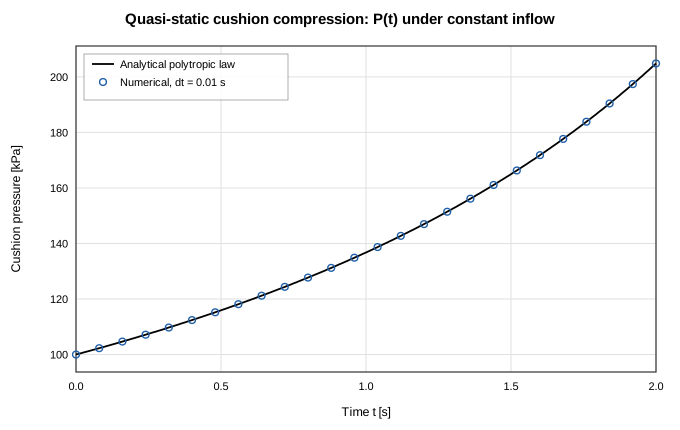
Figure 4-1. Verification of the cushion formulation: quasi-static compression under constant inflow against the analytical polytropic law. From docs/validation/fluid-transient-report.md.

4.6 Solution Procedure

4.6.1 Steady State

1. Unknowns — pressure at every internal node and mass flow rate in every branch; real-fluid networks add nodal enthalpy.
2. Residuals — mass conservation at each internal node and the momentum relation for each branch, assembled into one coupled system.
3. Jacobian — by default hybrid. Where every contributing code path is authored in TypeScript — the analytic EOS models and components with dual implementations (pipe, orifice, resistance, valve, bend, areaChange, checkValve, dynamicCheckValve, rectChannel, capillaryChannel) — derivatives are exact, computed by forward-mode dual numbers in a single residual evaluation per column. Note that dynamicCheckValve's ODE state (position) is frozen for the whole Newton solve, so its pressureDropDual is exact with respect to $\dot m$ exactly like valve's fixed-position case. Real-fluid networks are also analytic: cached $\partial(\rho,T)/\partial(P,h)$ partials are evaluated once per node per Jacobian build and chained through every column, so CoolProp calls scale with the number of nodes rather than nodes × columns. Finite differences remain only where the residual is genuinely non-differentiable — pump, regulator, reliefValve, orifice (when $Y$ is active), cavitatingVenturi, and heatedPipe branch heat get per-entry patches — and the whole matrix falls back to finite differences for unsupported configurations: species transport, and real-fluid networks carrying a gas cushion. Setting jacobian: 'fd' forces the pure finite-difference path.
4. Linear solve — dense Gaussian elimination.
5. Update — $\mathbf{x}_{n+1} = \mathbf{x}_n + \omega\mathbf{J}^{-1}\mathbf{R}$.
6. Zero-flow linearization — for $|\dot m| < 10^{-7}$ the branch relation is linearized about the threshold to keep the Jacobian non-singular. Components that are already smooth at zero flow (rectChannel, capillaryChannel) are evaluated exactly instead.
7. Convergence — declared when the residual norm is below tolerance. The residual mixes mass rows [kg/s] with momentum rows [Pa], so when the largest warm-start flow $F$ is below $10^{-3}$ kg/s the mass-flow rows (nodal balances and imposed-flow branches) are weighted by $10^{-3}/F$ (at most $10^9$) in both the stopping test and the line-search merit, so mass imbalances are judged relative to the flows present. Without this, a microfluidic compliance transient met an absolute tolerance at its warm start and froze. At or above $10^{-3}$ kg/s the weight is 1 and nothing changes; if round-off keeps the weighted bar out of reach, the step is accepted on the unweighted norm after at most three further iterations.
8. Globalization and PTC — for real-fluid problems the default inner-loop strategy is a trust-region dogleg in scaled variable space, computing the Newton step, the Cauchy point, and their dogleg intersection, and accepting on the actual-to-predicted reduction ratio; the radius grows on good agreement and shrinks on poor, with at most two retries per iteration, falling back to backtracking line search if dogleg fails. Real-fluid steady solves add pseudo-transient continuation: the direct Newton step is tried first, and only if globalization rejects it does the solver take a strongly regularized pseudo-transient step, with switched-evolution relaxation growing the pseudo-time step as the residual falls so that exact Newton is recovered at convergence. Non-real-fluid problems use the direct step with line-search acceptance. globalization: 'lineSearch' forces the legacy path everywhere.

4.6.2 Transient — Fixed Step

Marching from $t = 0$ to endTime in uniform steps of dt, each step:

1. Applies boundary, ambient, valve, and flow-source schedules at the new time.
2. Solves a steady-like coupled Newton system with storage added to the mass residual, $$R_{\text{mass},i} = \sum \dot m + \frac{\left(\rho_i^{n+1} - \rho_i^{n}\right) V_i}{\Delta t},$$ and internal-energy storage in the energy residual, $$\frac{(m^{n+1} c_v T^{n+1} - m^n c_v T^n)}{\Delta t} = \sum_{\text{in}} \dot{m} c_p T_{\text{upwind}} - \sum_{\text{out}} \dot{m} c_p T^{n+1} + \dot{Q}_{\text{in}}$$ The $c_v$ on the storage side and $c_p$ on the flux side are the correct pairing, not an inconsistency: stored energy is internal energy while transported energy is enthalpy (section 4.1.3). For networks outside the coupled [P, ṁ, h] mode this row is resolved implicitly for $T^{n+1}$ by successive substitution once the mass-flow field has converged.
3. Runs logic rules and controllers on acceptance, then stores the converged state. A step is certified converged only when the row-floor-scaled residual of its best Newton iterate is below $10^{3},\text{tol}$ — the same bar for every fluid model (converged steps sit at $10^{-5}$–$10^{-4}$, stalled ones at $0.1$–$10$). Two further conditions withdraw certification regardless of the residual: a real-fluid property evaluation that fell through to the last-resort fabricated state, and a reaction sub-step whose stiff integration failed — a step built on either is not a solution of the equations. Every step is appended to the trajectory even if the Newton did not converge; those steps are flagged converged: false and the per-step residual series stepResiduals / stepResidualsScaled record the raw and scaled norm that was achieved. Unlike adaptive stepping, fixed stepping never retries with a smaller $\Delta t$.

4.6.3 Transient — Adaptive Step

Adaptive stepping uses step doubling for local error control. Each candidate step takes one full backward-Euler step of size $\Delta t$ giving $y_1$, and two half-steps giving $y_2$. The weighted RMS error runs over every dynamic state: internal fluid-node pressures and temperatures (enthalpies for enthalpy-state fluids), solid temperatures, the mass flow of branches with fluid inertia (scaled by absTolMdot), and the integrated state of stateful components such as a dynamic check valve's opening. Those components are advanced along both candidate trajectories and rolled back when a candidate is rejected, so the step is a transaction over the complete state. The norm is

$$\text{err} = \sqrt{\frac{1}{N}\sum\left(\frac{y_2 - y_1}{\text{absTol} + \text{relTol}|y_2|}\right)^{2}}$$

The step is accepted when $\text{err} \le 1$, and the next size is

$$\Delta t_\text{new} = \Delta t\cdot\text{clamp}\left(0.9\text{err}^{-1/2},0.2,5\right)$$

clamped to [dtMin, dtMax]. A rejected step is retried smaller; if dtMin is reached the step is force-accepted and counted in stats.dtAtMinCount, which is the record that the tolerance was not met. Event alignment truncates the step so that every accepted step lands exactly on schedule breakpoints and on endTime. Adaptive runs report stats: { steps, rejectedSteps, minDt, maxDt, dtAtMinCount }.

4.6.4 Convergence Diagnostics

Convergence is reported, never assumed. Each run records a bounded solver diary built only from evidence that crossed the worker boundary — the throttled progress stream and the final result — and classifies the outcome as converged, not converged, stopped short, user-terminated, cancelled, or errored. Diaries account explicitly for what was retained and what was dropped; a diary synthesized from a bare final result is labeled finalEvidenceOnly rather than inventing progress milestones. Stall warnings are phrased in progress samples, not solver iterations, since that is what the evidence actually contains.

Known convergence behaviors, including coupled-residual certification and dome-edge limit cycles in real-fluid problems, are catalogued in docs/solver-convergence.md. Practical measures for a difficult case, in the order worth trying: supply better initial pressures and temperatures at internal nodes; reduce relaxation; increase maxIterations; subdivide long branches; for a steady real-fluid case seed nodes near the state you expect, including inside the dome if flashing is thermodynamically required; and for a closed ideal-gas loop introduce a small leak (section 1.7).

---

5. Program Structure

5.1 Modules

Module	Path	Responsibility
Core	src/core	Schema, decoding, validation, EOS, components, correlations, steady and transient solvers
Substrate	src/substrate	.fn text projection: serialize, parse, line mapping
Interface	src/ui	Canvas, panels, run history, sweeps, diary, worker client
Worker	src/ui/solverWorker.ts	Off-main-thread solve execution
Companion server	scripts/serve.ts	Serves the built app; discovers and creates component files
Validation corpora	src/validation	Published benchmark data and digitized traces

The core has no DOM, React, or worker dependency. Module boundaries, public versus internal API, configuration lifecycle, and test tiers are described in docs/architecture.md.

5.2 Configuration Lifecycle

Every solve, whether from the interface or a script, passes through the same pipeline:

untrusted input
  → decodeNetworkConfig        structural decode; version 2 only
  → resolveNetworkParameters   formula bindings resolved to numbers
  → validateResolvedNetwork    fluid, nodes, solids, species, settings,
                               branches, conductors, logic, controllers,
                               component library, closure parameters
  → solveSteady / solveTransient

There is no path that reaches a solver without decoding and validation.

5.3 Solver Worker

The solver runs in a dedicated Web Worker so that a long solve never blocks the interface. The main thread posts {type:'run', config, mode}; the worker replies with ready, coolpropLoading, progress, done, or error.

Progress payloads are cheap partial snapshots — arrays sliced to the current length, so each emission costs on the order of the number of tracked variables rather than the whole history — and are throttled to at most ten per second to bound structured-clone overhead. solveTransient emits every $\max(1, \lfloor \text{totalSteps}/200 \rfloor)$ steps by default.

Because the solve loop is synchronous, a posted cancel message cannot be observed mid-iteration without SharedArrayBuffer, which the application avoids since it would require cross-origin isolation headers. Cancellation therefore terminates the worker and respawns a fresh one on the next run. Cancelled runs keep whatever partial trajectory was already delivered, clearly labeled as partial.

5.4 Real-Fluid Sidecar

When any fluid spec is realFluid, the worker initializes CoolProp itself, once per worker rather than once per substance. The WebAssembly module is imported dynamically, so networks that never touch a real fluid never pay for it. Everything else — validation, all analytic EOS models, both solvers, and the .fn format — is pure TypeScript with no external dependency.

5.5 Using the Core as a Library

From Python, pip install openflume provides the same core with no JavaScript toolchain. The equivalent of the steady snippet below is openflume.load("network.json").solve(). See Python package. The rest of this section covers TypeScript use.

The supported export surface is src/core/index.ts. The package is not yet published to npm, so import from the source tree as the tools under scripts/ do. The snippets below are written that way and work as typed from a script beside src/; adjust the relative depth to match where you put the file. Once the package is published the same imports become from "openflume/core", with nothing else changing. Run scripts with npx tsx script.ts on Node 22.9 or newer. The DynamicCheckValve constructor is currently exported from src/core/components rather than the supported core barrel; construct it through NetworkConfig like the other components.

Steady solve:

import { solveSteady, validateNetwork, decodeNetworkConfig } from "../src/core";
import { readFileSync } from "node:fs";

const config = decodeNetworkConfig(
  JSON.parse(readFileSync("network.json", "utf8")),
);

const errors = validateNetwork(config);
if (errors.length > 0) {
  console.error("Invalid network:", errors);
  process.exit(1);
}

const result = solveSteady(config, {
  onProgress: ({ iteration, residual }) =>
    console.log(`Iter ${iteration}: residual = ${residual.toExponential(3)}`),
});

console.log("Converged:", result.converged, "in", result.iterations, "iters");

Transient solve:

import { solveTransient } from "../src/core";

const result = solveTransient(config, {
  onProgress: ({ time, endTime, dt }) =>
    console.log(`t = ${time.toFixed(3)} / ${endTime} s (dt = ${dt} s)`),
  shouldAbort: () => false,
});

console.log("Recorded steps:", result.times.length);
console.log("Tank pressure trace:", result.nodes["tank"].pressure);

Real fluids must be initialized once before solving:

import { initRealFluids, solveSteady } from "../src/core";

await initRealFluids();
const result = solveSteady(realFluidConfig);

Passing shouldAbort lets a caller stop a run early; the returned result carries the partial trajectory with aborted: true. Always check result.converged before using numbers — the solver returns its best state either way, and it is the caller's job to notice.

5.6 User-Authored Components

Two extension routes require no code at all: dpTable for tabulated pressure drop and customResistance for a constant or Reynolds-dependent loss coefficient. Beyond those, a component may be authored in JavaScript.

Local component files live under library/components/ as *.component.js, each calling defineComponent({ metadata, pressureDrop, heat }) exactly once, with no imports or exports. With the companion server running, the application discovers them, lists them as named palette entries, and lets branches reference them by name with declared parameter defaults. The + Create custom component entry in the connection chooser opens an authoring form that validates and previews the generated source and then asks the server to write the file; the server refuses to overwrite an existing one. Four worked templates ship in library/.

Alternatively, source may be embedded directly in the model under componentLibrary, which keeps a model self-contained at the cost of carrying executable code inside a data file. Loading a model with embedded code that does not match a previously approved hash requires explicit consent.

This is a trust model, not a sandbox. Component code runs through new Function with full access to the page. Treat library/components exactly as you treat src/. The complete contract is in docs/usercode.md.

---

6. Graphical User Interface

6.1 Workspace Tabs

Beneath the toolbar, a tab strip selects the workspace:

Tab	Contents
Model	The P&ID canvas — the default view
(subnetwork tabs)	One closable tab per opened group, showing only its members plus ghost ports for cross-boundary connections
Setup	Everything global about the model: solver, physics, fluids, species, units, extensibility
Sweep	Session-only parameter-sweep workspace
Results	Channels explorer, result tables, run history, solver diary

To the left, the Project outline lists the whole project — the active variant's configuration and elements, plus every recorded run — and can be hidden with Ctrl/Cmd+\. To the right, a docked Properties panel appears whenever something is selected and gives its width back to the canvas otherwise; drag its left edge to resize it. See §6.11 for the outline and §6.12 for simulation variants.

6.2 Toolbar

The network name field doubles as the save-file name and shows a dot when there are unsaved changes. New, Save, and Load handle .fn files; Undo and Redo walk the history. Load opens any file the editor can hold — including a half-finished model the solver would still reject (no boundary node yet, a transient without volumes), whose remaining issues then show in the health pill. Only files that are not a network at all, or whose element references dangle, are refused. Examples ▾ lists the fourteen shipped models in four groups. Units ▾ selects the display preset — SI, Metric engineering, or US customary — and shows a disabled Custom entry when preferences match no preset. Commands (or Cmd/Ctrl+K) opens the command palette, which can run the model, place elements, switch views, and jump to any element by id.

When a simulation variant other than Base is active, its name appears as a pill beside the network name — so the variant you are editing stays visible even with the project outline hidden.

Run starts a solve; while running the button becomes Running… with a Cancel beside it, and live progress reads Iter … · residual … for steady or t = … s / … s · dt = … s for transient.

A status pill to the right reports the current health of the model and the last run: Ready to solve, N issue(s) to fix, Solving…, Converged or Not converged with iteration count or step count, Cancelled, or a separate Fluid init failed if CoolProp could not start. A stale suffix means the model has been edited since the displayed result was computed.

6.3 Canvas Tools

The left rail is organized in sections.

Canvas tools. Select enables marquee multi-selection; Pan is the default drag behavior. Inspect properties reads every available result property off the selection after a converged steady or transient run. Schematic view / 3D view toggles between the P&ID layout and placement by physical position; the 3-D view adds Iso, Front, Top, and Side presets, with drag to orbit and right-drag to pan. Hide labels / Show labels toggles names and solved readouts. View options filters what is drawn — fluid nodes, thermal nodes, fluid branches, and conduction, convection, or radiation ties independently — which is how a large conjugate model becomes legible.

Fluid nodes. Internal node and Boundary node.

Thermal nodes. Solid node and Ambient node.

Annotations. Text note.

Model views. Text view and Table view open the corresponding dialogs (section 6.10).

At the top right, Color by selects the quantity painted onto the diagram. The list is generated from the same channel registry that feeds the plots and result tables, so it offers every quantity a result can carry: Pressure, Temperature, Density, Enthalpy, Internal energy, Entropy, Specific heat, Viscosity, Thermal conductivity, Speed of sound, Gas volume, Quality and Front fraction for nodes; Mass flow, Pressure drop, Velocity, Volumetric flow, Mass flux, Dynamic pressure, Reynolds and Mach for branches; Heat rate, Heat flux, Heat transfer coeff and Wetted fraction for conductors — plus None. A shared blue-to-red colormap is used, with a legend directly beneath the selector showing the quantity, unit, and domain; elements to which the quantity does not apply are muted. Before a run, or when a result is stale, colors show initial and boundary conditions; after a steady run they show the converged field; after a transient run they follow the time scrubber. A Global map overview at the bottom right can be expanded or collapsed.

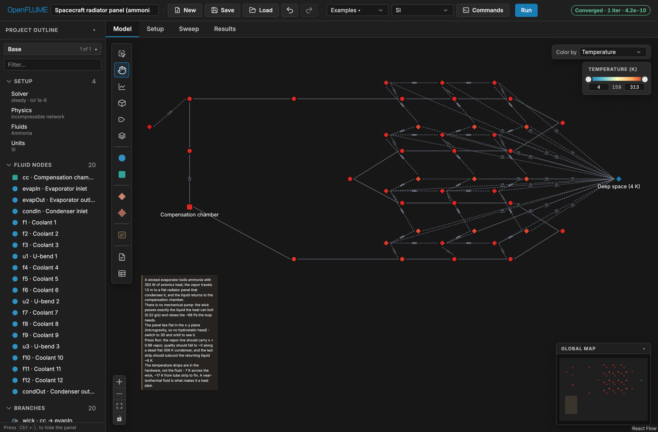
Figure 6-1. Color by Temperature after a converged run, with the shared colormap legend at the top right.

6.4 Building a Circuit

To place a node, click its rail tool — the element appears at the viewport center, snapped to the grid — or drag the tool onto the canvas to place it at the pointer.

To create a branch or conductor, there are two gestures, and which one you use decides when the component type is chosen.

Drag from a handle. Drag from one node's connection handle to another. On release, a Connect with chooser lists the available component types grouped as common flow, advanced flow, custom flow, and Thermal ties, plus + Create custom component and a refresh control for local components. Choosing an entry creates the connection with that component's default parameters and selects it for editing. Cancel or Escape dismisses the chooser. The chooser appears only when no palette tool is armed — arming a tool has already answered the question it asks.

Click, then click. Arm a component in the palette, then click a source node and click a target node; the connection is created immediately with the armed component's defaults, and the tool stays armed for the next one. A hint banner appears at the top of the canvas — first click a source node, then click a target node to connect, then, once a source is taken, now click the target node — so the pending endpoint is always visible. Clicking the armed source node a second time releases it.

While a tool is armed, the connection handles on eligible nodes only — not every node — grow from 5 px to 7 px and take a gold outline (--select, #c99a43), which is the same colour the interface uses for selection. Before a source is picked, eligible means "can start this kind of connection"; after one is picked, it means "is a legal partner for that source". Ineligible nodes are left alone, so the highlight is a live map of where the connection may go.

Escape unwinds one level at a time, in order: an open chooser, then a member picker, then the pending source node, then the armed tool itself. Clicking empty canvas also drops a pending source (and clears the selection) but leaves the tool armed.

Connection rules are enforced on creation, with a red banner explaining any rejection: fluid branches join only fluid nodes; conduction and radiation conductors join only thermal nodes; a convection conductor requires exactly one fluid endpoint and one thermal endpoint. The banner does not auto-dismiss; the next interaction clears it.

Dropping or clicking a connection onto a group container prompts with Select member node when more than one member qualifies, and connects straight through when exactly one does.

To select, click an element; shift-click adds to the selection, and the Select tool allows marquee selection. A selection-actions menu offers Duplicate, Repeat… (chain the selected unit into N series instances — section 3.13), Split… (divide a selected pipe or heated pipe into N equal series segments — section 3.13), Create subnetwork, and Delete.

Groups. Select two or more nodes and create a subnetwork; a colored container appears. Double-click the container — or use Open Tab in its property panel — to open its tab and work on members in isolation, with ghost ports standing in for cross-boundary connections, which are drawn dashed on the main canvas. Ungroup returns members to the main canvas with positions preserved. Groups never affect results.

Notes. Place the note tool and type. Double-click to edit in place — Escape discards, Cmd/Ctrl+Enter commits. A note grows with its text until the corner handle is dragged, which pins an explicit box that the text then scrolls inside; clearing Width or Height in the panel returns to fitting the text. Notes inside a subnetwork tab stay pinned there.

6.5 Property Panel

With nothing selected the panel reads Select a node, branch, or group to edit properties. Otherwise it is titled for the selection — Node, Solid Node, Branch, Conductor, Subnetwork, Note, or N selected.

Fluid node. Label, Type (Internal / Boundary), Subnetwork, Fluid when named fluids exist, Position (m) as X/Y/Z, then conditions: Pressure, Temperature, Volume for internal nodes, Trapped gas cushion with Initial Gas Volume and Polytropic Index (1.0–1.4), and Heat Input. Boundary nodes add Pressure Schedule and Temperature Schedule tables. Diagram X/Y are separate from physical Position (m).

Real-fluid nodes add a State variable selector of Temperature or Vapour quality. The two are mutually exclusive (section 3.4), so choosing one replaces the other's field and clears its value; quality is not offered for the analytic fluid models, which have no saturation dome. When some convection conductor opts into cryogenic front transport, boundary nodes also gain Cryogenic front inlet on [0,1] — 1 marks a cryogenic inlet, blank or 0 a warm boundary. When the network declares species, every node gains a Composition group of one mass fraction per species with a running sum and a Normalize to 1 action; partial entry is allowed, and the sum has to reach 1 to solve.

An internal node also exposes Reacting junction (combustor). Enabling it selects the CEA propellant pair and efficiency, the named ideal-gas product fluid, and the oxidizer/fuel role of each inbound branch. Validation enforces the kineticEnergy (and, in transient mode, positive-volume) restrictions described in section 3.9.2.

Solid node. Label, Type (Solid / Ambient), Subnetwork, Position (m), Temperature, Mass and cp for solids, and Heat Input. Ambient nodes add Temperature Schedule. The cp field exposes all five specific-heat modes, showing the source and validity range inline for catalogue materials.

Branch. Label, From, To, Initial flow guess, and Component Type grouped as Common, Advanced, and Custom, followed by the parameters for the chosen type (Appendix A). From and To are dropdowns, not labels: selecting a different node retargets that endpoint in place, keeping the branch's id, label, and component parameters. The list is organized by subnetwork, so an endpoint can be moved across a group boundary — into a group, out of one, or between two — without deleting and redrawing the branch. Conductors expose the same retargeting on their own From and To, filtered to endpoints legal for the conductor kind. Initial flow guess is the Newton warm start initialMdot; left blank it reads Auto (0.1 kg/s) and never constrains the converged solution — with one exception: a transient pipe with Fluid inertia enabled uses it as the actual ṁ at t = 0 in its (L/A)·dṁ/dt term, so there it is an initial condition and should be set to the real starting flow (0 for fluid at rest behind a closed valve).

Pipes carry a Friction selector of Correlation (Swamee–Jain) or Constant f. The constant form is a separate mode rather than a bare number because absent and zero mean different things: frictionFactor: 0 is a frictionless pipe, so an emptied field must not read as one. A Tapered outlet checkbox reveals Outlet Diameter (diameterOut); friction uses the mean diameter, and the hint says whether the endpoint areas are currently feeding the acceleration and kinetic-energy terms. Heated pipes add a Boiling model selector of UA·ΔT only or Miropolskii film boiling. Splitting a pipe or heated pipe into segments is an action, not a property: select the branch and choose Split… from the canvas selection-actions menu — length, elevation change, and $UA$ are divided across the segments rather than duplicated (section 3.13).

A customResistance branch edits its K(Re) curve in place, as a Reynolds/K point grid beside a readout of the point count, the Reynolds span, and the K the last solve interpolated. A constant K can be promoted with Make K depend on Reynolds — seeded flat, so promotion changes the shape of the closure without changing K — and a table collapsed back with Replace with constant K. Only the table form needs Diameter (that is what makes Reynolds computable), so a constant-K branch offers + Add diameter instead.

Conductor. Label, From, To, and Kind, then kind-specific parameters. Convection conductors expose a heat-transfer-model editor with per-model inputs and suitability warnings.

Subnetwork. Label, position, member count, Open Tab, Ungroup.

Note. Text, X, Y, Width, Height, Delete note.

Multi-selection groups the selection by kind and bulk-edits shared numeric fields, marking differing values Mixed. Labels, endpoints, schedules, gas cushions, property specs, convection models, and physical positions are excluded from bulk editing.

After a run, a results block reports the solved values for the selection — every quantity the result carries for that element, as listed in section 6.8 — tagged stale if the model has since changed.

Formula-capable fields carry the f(x) button described in section 3.10.

6.6 Setup

The Setup tab holds everything global about the model — everything that is not the network itself — in six sections: Solver, Physics, Fluids, Species, Units, Extensibility. It always opens on Solver, and leaving the tab returns it there, so the basics are one click away and the advanced surfaces stay out of the way until you want them. Rows in the project outline's Setup section open this tab directly on the section they name.

These settings belong to the active variant (§6.12): editing them while a variant is active records the change into that variant, exactly as editing an element does.

Solver sets Mode (Steady / Transient), Tolerance, Max Iterations, and Relaxation; in transient mode it adds the time-stepping choice of Fixed dt or Adaptive, with Time Step and End Time for fixed stepping and Min dt, Max dt, Initial dt, Relative tolerance, Safety factor, and the two absolute floors Absolute pressure tolerance and Absolute temperature tolerance for adaptive. An Advanced numerics disclosure holds the Newton strategy: Steady solver (pseudo-transient continuation or direct Newton, steady mode only), Globalization (trust region or line search), Jacobian (hybrid analytic/FD or finite difference), and the experimental Re-certify after coupling. The defaults suit every shipped example; reach for these only when a solve will not converge.

Physics holds the compressible formulation. Momentum flux adds the convective-acceleration term and Kinetic energy switches branch transport to stagnation enthalpy; together they make the network quasi-1-D. A derived summary line names the formulation the current combination selects, so the interaction between the flags is visible rather than inferred. Momentum-flux scheme (limited upwind or central) is disabled until momentum flux is on, and the Second-law admissibility audit — on by default — is enabled only for the steady central-scheme case it applies to. A Closure calibration disclosure exposes the empirical constants of the Dittus–Boelter, Miropolskii, and Swamee–Jain correlations plus the solidCpScale material multiplier; each field shows its published default as a placeholder, and clearing a field returns the network to the published value rather than writing it in. Solver numerics are structurally unreachable from that surface (see core/closureParams.ts).

Fluids is a single roster: the default fluid is the first card, and + Add fluid appends named isolated continua. Every card — default and named alike — offers the same editor: a model of Incompressible, Ideal Gas, Expandable Liquid, or Real fluid (CoolProp), then either a preset (Water, Air, Water Expandable, shown read-only) or Custom, which seeds the preset's constants into editable fields (rho, mu, cp and the model's other parameters, plus arbitrary extra keys). Real fluids replace the preset with a searchable 124-fluid catalogue (favorites first, then search by name, alias, or CAS, with warnings for no-transport and unknown names).

Species turns multi-species transport on and off. The roster is a table of species names and molecular weights, with optional whole-column properties for specific heat, formation enthalpy, and viscosity (whole-column because the solver rejects a ragged set). Beside it, the reaction list edits Arrhenius reactions: stoichiometry is entered per declared species, so a reaction can never name a species the roster does not have, and each card shows its equation as it is built. Removing the last species removes the block, and node mass fractions that named a departed species go with it. Species transport requires a single ideal-gas continuum; the tab says so when the network cannot support it.

Units selects the display preset and per-quantity preferences. Extensibility holds the registers, logic-rules, and controllers JSON editors.

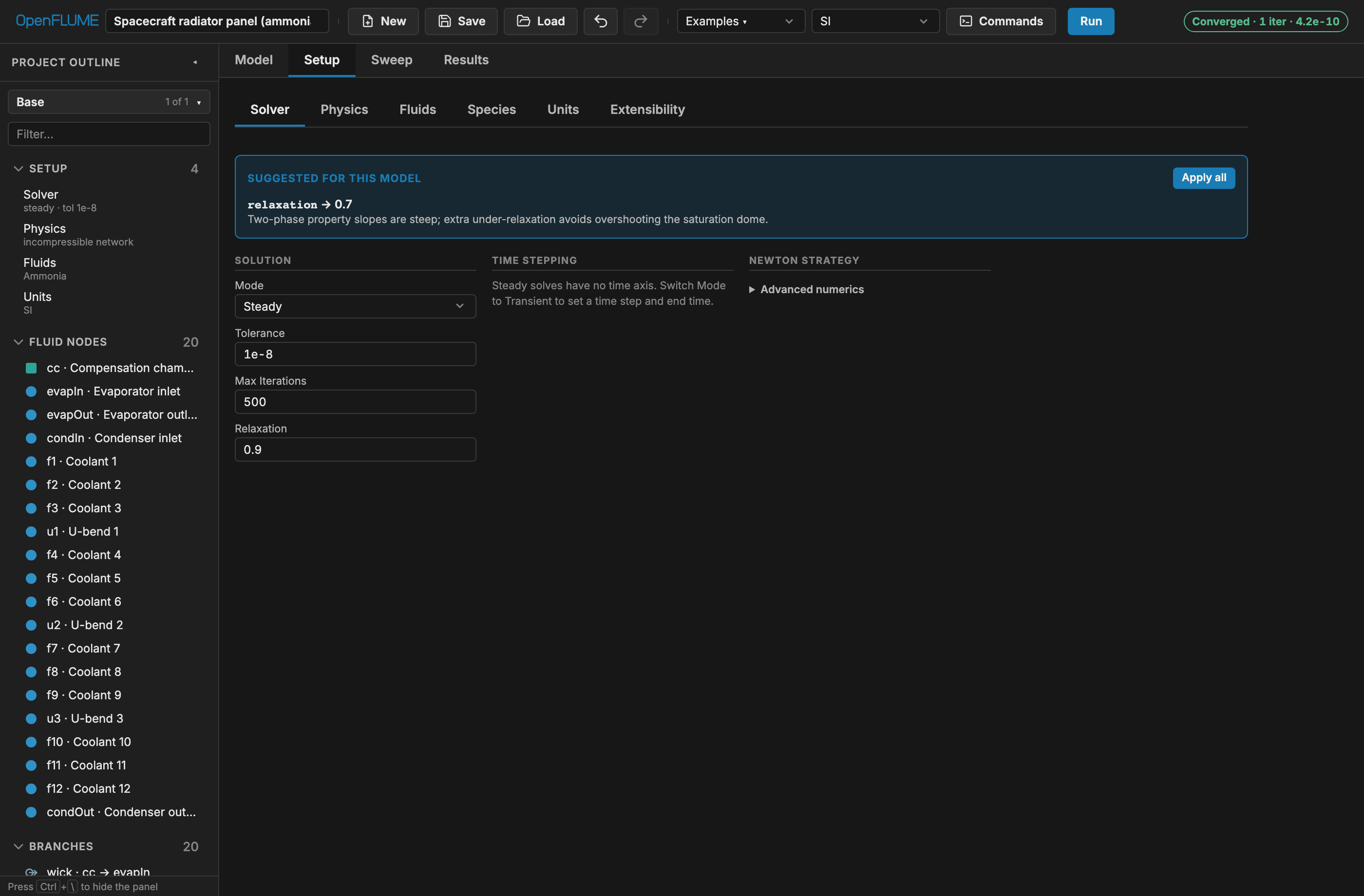
Figure 6-2. The Setup tab on its Solver section: the section tabs across the top, solution tolerances on the left, time stepping in the center, and the Advanced numerics disclosure on the right.

6.7 Running a Model

Click Run. Validation runs first, and a model with issues will not solve — the status pill shows the count and opens a list in which each issue selects the offending element on the canvas. Progress appears in the toolbar. If the Results tab is open with channels plotted, those series update live as transient steps complete. Cancel terminates the run and keeps the partial trajectory, labeled as partial.

6.8 Analysis (Results Tab)

The Results tab is where results are read. The tab's title is the run selector: it names the displayed run and switches between Latest run and each historical run, with the outcome badge, the run's evidence (iterations or accepted steps), and any partial or baseline pill beside it. There is no separate strip above it repeating the same facts. Banners announce a failed run, a stale result — Results are from an earlier model state. Rerun before using these values for a design decision. — or a cancelled partial.

Everything else about the run — the solve summary, the result tables, the solver diary and the run history — sits in the collapsible sections below the plots, each opened from its own header.

Plots

The Results tab holds plots, one per tab. A plot is two things and nothing else: an x axis and a list of channels. Add as many plots as you like with + Plot — pressure along the feed line in one tab, tank pressure over time in another — rename a tab by double-clicking it, and close it with its ×. Plots survive leaving the Results tab and are cleared when a different model is loaded.

A new plot is empty. Nothing is pre-selected, because which of the several hundred channels a result carries matters to you is not something the tool can guess.

Choosing the x axis

Axis	What runs along the bottom
Time	The transient sample axis (transient results only)
Station along path	Distance through the network along a chosen flow path
Position X / Y / Z	The element's physical coordinate in metres
Element order	Position in the model — the axis that always exists

The axis decides what a channel means on the plot, and the difference matters:

• On Time, a channel is a series. Three node pressures draw three lines, each tracing one element through the run.
• On every other axis, a channel is a point. Three node pressures draw one line across the network, because the thing varying along the axis is the element, not the sample. Channels are grouped into a line per quantity, so pressure and temperature are two lines on their own scales.

Plotting node pressures against Station along path is therefore the hydraulic grade line: you see not just that pressure was lost but where. A Path selector appears with that axis, offering every route the solved flow supports — one per outlet of a tee, one per stream of a counterflow pair, or a closed loop where the network circulates.

Flow direction is not declared in the model: a boundary node is a reservoir and a branch's drawn from → to is only a sign convention. OpenFLUME orients the network by the solved mass-flow signs and walks it downstream from wherever mass enters, so reverse flow is drawn the right way round.

Quantities that belong to a span rather than a point — a branch's mass flow or pressure drop — are drawn as stairs on a spatial axis, because a component's value does not vary along itself.

The axis degrades honestly. Station is a real distance when every component on the path carries a length (or its endpoints carry physical positions), and a station index that says so when even one does not. Element order is always an index. An element with no coordinate on the chosen axis is left out and named, never placed at zero.

Choosing channels

What the plot currently draws is listed in a Plotted block at the top of the picker, with each channel's value and an × to drop it, so the answer to "what am I looking at" is never somewhere down a scrolling list. Clear empties the plot.

Below it, the picker lists every channel the result carries, narrowed by three controls on one line:

• a search box;
• sort (the bars glyph) — group the list by quantity, the default, or by element;
• filter (the funnel) — restrict it to fluid nodes, branches, solid nodes or conductors, each option carrying the glyph the canvas draws for it.

Each row shows its current value in your display units and its element's canvas glyph; clicking it adds or removes it from the plot and selects that element in the model. The or plot a whole set… control fills the plot with a whole family in one go — every node pressure, every branch mass flow, and the other sets listed in §6.8.

Comparing runs on one plot

The question a design study asks is "which one was better?", and flipping between two runs a second apart cannot answer it. Above the chart, a Results row names the run the plot is reading — the one chosen in the title dropdown — and + Compare run… overlays another recorded run on the same axes. The same channels are resolved against each run, so adding a run doubles the lines rather than changing what is drawn.

Overlaid runs are dashed and keep the colour of the channel they mirror, so the eye groups by quantity first and tells the runs apart second; every series is labelled with the run it came from. Each overlay is resolved against its own captured model, so a variant that moved a node or lengthened a pipe is plotted on the geometry it actually ran, and its values are interpolated onto the plot's axis rather than read off by sample index — two runs on different timesteps still line up. Where an overlay has no data (a coordinate the other run's axis never reaches, or a steady run on a time axis) the line simply stops; nothing is extrapolated.

The comparison belongs to the plot, not the tab: one plot can hold a two-design comparison while the next reads the latest run on its own. Up to four runs can be overlaid on one plot. Drop one with the × on its chip. A pinned baseline run (§6.12) is overlaid on every plot the same way, without being added by hand.

Findings

Under the plot, deterministic readings of the result appear when there is something to say — the component that dominates the pressure drop, branches running backwards, near-sonic or sonic flow, mass that does not balance at a steady junction, and any advisory the solver itself raised. Each states the numbers behind it and selects the element it is about. Nothing is shown when there is nothing to report; silence means the result reads cleanly.

Exports

Export CSV writes the current plot's channels with provenance; Export all writes every result channel. A transient export is a plottable table — time is the first column, each channel is its own column headed by its label and unit, and a channel with no finite sample at some instant leaves that cell blank rather than shifting the column. A steady export, having no time axis, is one row per channel. Every chart also exports itself as PNG, SVG, or CSV with the run's provenance in the footer.

6.9 Parameter Sweeps

The Sweep tab explores one scalar parameter at a time and is deliberately session-only: jobs are never written to the model file or to browser storage.

Under Define a sweep, pick a Sweep target from the grouped list of settings, fluid node, solid node, branch, and conductor fields — with a filter box for large models — then set Start, End, and Variants (1 to 25, inclusive linear spacing). Values are entered in config-native SI units regardless of display preset. Run Sweep creates and starts the job; Create defines it without running; New sweep resets the form.

Variants solve strictly sequentially in the solver worker. A failed variant is recorded and the sweep continues. Each job solves a frozen, hashed snapshot of the model, so later edits raise a staleness banner rather than silently changing what is being compared, and a sweep never touches the model, the text buffer, undo history, or autosave. Per-job controls include Start, Cancel, Rerun incomplete, Rerun all, Discard, and Export CSV.

The variant table reports value, status, convergence, solve detail, diary event count, peak absolute mass flow, pressure and temperature ranges, and duration. Promote on a completed row creates a saved simulation variant named after the swept value, with the swept field as its patch and the promoted run filed under it — how a sweep finding becomes something that survives the session.

6.10 Model Text and Model Table

Text view opens Model Text, a full-workspace source editor over the same lossless text projection used by .fn files. Keystrokes stay local until Apply (Cmd/Ctrl+Enter), which commits valid text as exactly one undoable history entry; invalid text is kept with line-level diagnostics in a Text problems region and never reaches the model. Selection syncs with the diagram in both directions.

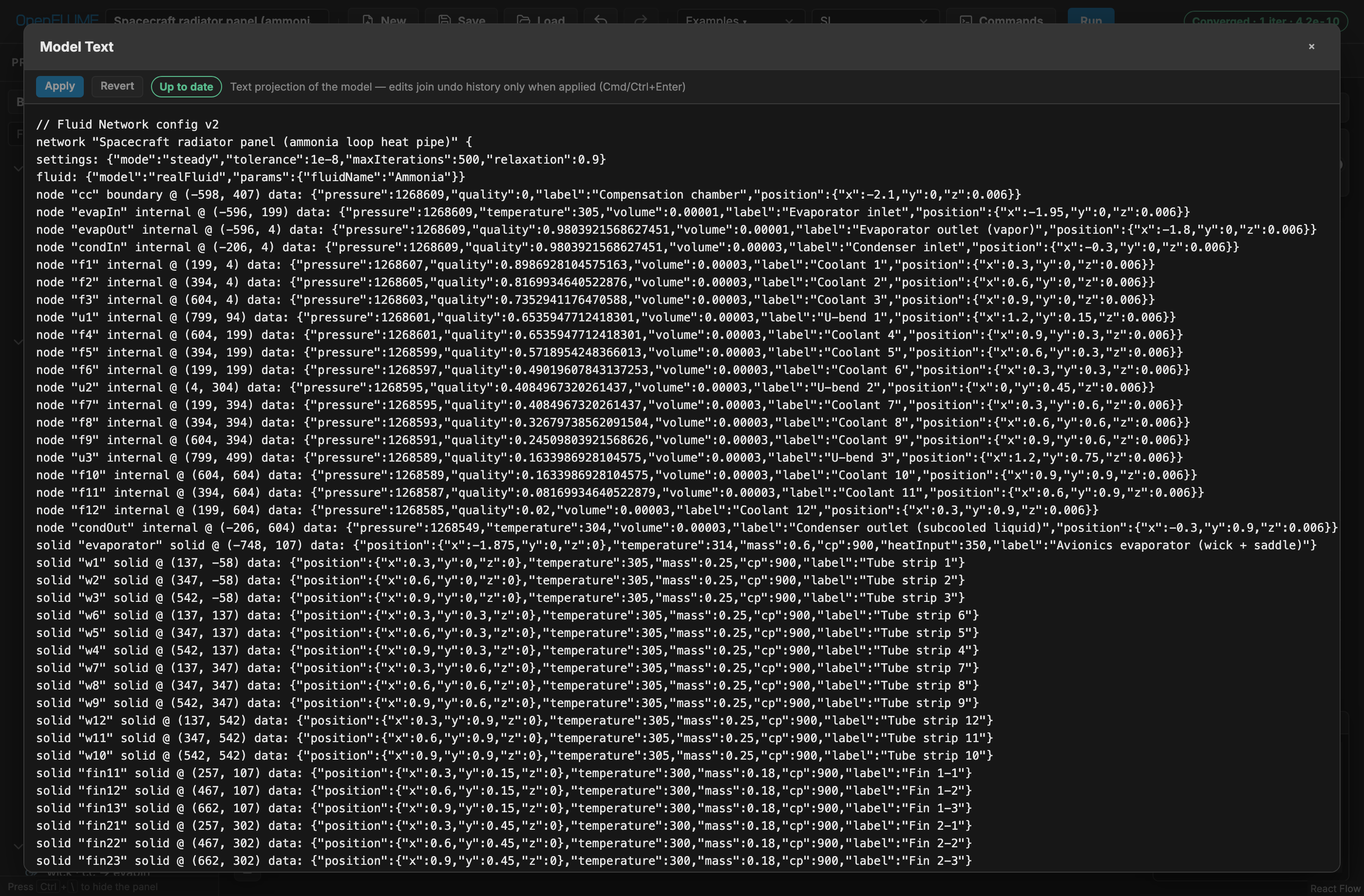
Figure 6-3. Model Text over the spacecraft radiator panel example: the same lossless text projection used by .fn files, with Apply and Revert in the header and an up-to-date status pill.

Table view opens Model Table, a tabular listing of every element, including a searchable Notes table, with a validation summary pill.

6.11 Project Outline

The left panel is a searchable tree over the whole project. Ctrl/Cmd+\ hides and shows it; a filter box narrows every section at once.

At the top sits the variant picker (§6.12), which both switches the active variant and labels everything below it as belonging to that variant. Beneath it:

• Setup — Solver, Physics, Fluids (with one child row per named fluid), Species, Units and Extensibility, each annotated with its current value. Clicking a row opens the Setup tab on that section.
• Element sections — fluid nodes, branches, solid nodes, conductors, subnetworks and notes. Each row carries the same symbol the canvas draws: a circle for an internal node, a rounded square for a boundary, a diamond for a solid (dashed when ambient), and the component's P&ID glyph for branches and conductors. Clicking a row selects the element and brings it into view on the canvas.
• Results — every recorded run, newest first, tagged with the variant that produced it (§6.12).

Hovering any element row opens an instant summary card: what the element is, its endpoints, the two or three parameters that define it, and — when a run is displayed — its solved values.

A row that needs attention carries an icon at its right edge: an amber triangle when a readiness check flags it, a red circle when a validation error names the element. Healthy rows carry nothing — fine is the default state, so the panel reads as a quiet list with the problems standing out of it. A collapsed section shows the worst icon among its rows, so a problem is never hidden by collapsing.

Elements can be dragged into a different order within their own section. Ordering is presentation: it round-trips through the .fn file and is undoable, but it never marks results stale, because listing the same network in a different order does not change the network. Reordering is disabled while the filter is active, since the visible rows are then not the full list.

6.12 Simulation Variants

A model file can carry named variants — alternative versions of the same network, differing in solver settings, parameters, or topology. The file body is the implicit Base variant; each additional variant is stored as a sparse patch recording only what it changes, so edits to the base flow through to every variant that does not override them.

The variant picker at the top of the outline switches between them and offers New variant from current, plus rename, duplicate and delete on each row. Creating a variant while another is active branches from that one.

While a variant is active, every edit is recorded into its patch and the base network is left untouched — every edit except the model name, which identifies the file rather than the network and always edits the base. Rows the variant overrides are marked M, with the base value in their hover card, and the picker shows how many changes the variant carries. Because the variant name also appears in the toolbar, the variant you are editing is visible whether or not the outline is open.

Variants are saved inside the .fn file, so they travel with the model.

Runs and comparison. Each run is filed under the variant that was active when it started (switching variants while the solver is busy does not move it) and shown in the outline's Results list with that variant's name. Click a run to display it; click the star beside another run to pin it as the comparison baseline, and that star stays gold for as long as the pin holds. The baseline may come from a different variant, which is how variants are compared: the delta columns and the dashed chart overlay then show one variant against the other.

Loading a different model clears the run list — results belong to the model that produced them.

Saving results. Results are not stored in the .fn file — that file stays a model description. They are mirrored into browser storage so an ordinary reload keeps them — editing the model in between does not lose them; restored runs whose model has since changed simply show as stale — and they are written to a portable <model>.runs.json sidecar beside the model. Save in the toolbar writes both files whenever there are runs to save, so one action captures the whole session; Save in the Results section header writes the sidecar alone. Loading a .runs.json through Load reattaches its runs to the open model. Saving always writes the whole file — the base network and every variant — not only the variant currently on the canvas.

Discarding results. Click the × beside a run to discard that one, or Discard in the Results section header to drop the whole list. Both ask for confirmation first, naming what will go, because discarding is permanent: it is not covered by Undo, and it clears the browser-storage copy too, so a reload will not bring the runs back. Save the sidecar first if the results matter. The model itself is never touched.

Promoting a sweep point. Promote in the Sweep workspace (§6.9) turns an interesting sweep variant into a saved simulation variant named after the swept value, with the swept field as its patch, and files the run under it.

6.13 Keyboard Shortcuts

Shortcut	Scope	Action
Ctrl/Cmd+Z	Global	Undo
Ctrl/Cmd+Shift+Z	Global	Redo
Ctrl/Cmd+D	Global	Duplicate selection
Ctrl/Cmd+K	Global	Open the command palette
Ctrl/Cmd+\	Global	Show or hide the project outline
Ctrl/Cmd+G	Canvas	Create subnetwork from selection
Delete / Backspace	Canvas	Delete selection
Escape	Canvas	Cancel connection chooser, picker, or pending action
Escape	Dialogs	Close dialog
Ctrl/Cmd+Enter	Model Text	Apply edits
Arrow keys	Focused chart	Step the chart cursor

Within a text field, Ctrl/Cmd+Z applies to that field rather than to model history.

6.14 Validation Messages

Validation runs continuously, debounced, on every model change, and again before any solve. Issues surface in four places: the toolbar status pill, whose popover lists each issue and selects the offending element when clicked; the Model Table summary pill; line-level diagnostics in Model Text; and transient red banners on the canvas for rejected connection attempts. CoolProp start-up failure is reported separately as Fluid init failed, since it is an environment problem rather than a model defect.

---

7. Example Problems

Thirteen models ship with the program, reachable from Examples ▾. They are grouped by intent: Verify-by-inspection cases whose answers can be checked by hand, Applications showing engineering use, Benchmarks reproducing published results, and Extensibility cases exercising logic, registers, and controllers.

Loading an example replaces the current network, so save any work first. Every example is a plain NetworkConfig, so the productive way to start a model of your own is to load the nearest example and edit it.

7.1 Sanity: Orifice Hand-Calc

Verify-by-inspection · steady · incompressible

Problem. Water at constant density flows between two fixed-pressure boundaries through a single orifice.

Model. Two boundary nodes, one orifice branch. The expected answer is written on the canvas as a note.

Check. The solved mass flow must match $C_d A \sqrt{2\rho\Delta P} \approx 0.8485$ kg/s within 0.5 %. This is the smallest case that exercises the whole chain — decode, validate, assemble, Newton solve, report — so it is the right first thing to run after any change to an installation.

7.2 Three-Pipe Junction

Applications · steady · incompressible water

Problem. The classic split-flow problem: one inlet at 300 kPa feeds a junction that discharges through two pipes to two lower-pressure outlets.

Model. Four fluid nodes — one inlet boundary, one internal junction, two outlet boundaries — joined by three pipe branches of differing length and diameter. Tolerance 1×10⁻⁹, 500 maximum iterations, relaxation 0.9.

Check. Inflow must equal the sum of the two outflows to solver tolerance, and the junction pressure must lie between the inlet and outlet pressures. The smaller-diameter leg must carry less flow. This is the case to modify first when learning the program: change a diameter and watch the split move.

7.3 Tank Blowdown

Applications · transient · ideal-gas air

Problem. A 0.1 m³ tank of air, initially at 500 kPa and 300 K, vents to atmosphere through an orifice over 5 s.

Model. One internal node with volume, one ambient boundary node, one orifice branch. Fixed step of 0.01 s.

Check. Tank pressure decays monotonically toward 101 325 Pa. Tank temperature must fall substantially below 300 K, because the internal-energy storage formulation captures adiabatic expansion cooling — for an ideal gas, $T \propto m^{\gamma-1}$. A model that holds the tank at 300 K throughout has lost the flow-work term. Discharged mass agrees with a Runge–Kutta reference to 0.5 %.

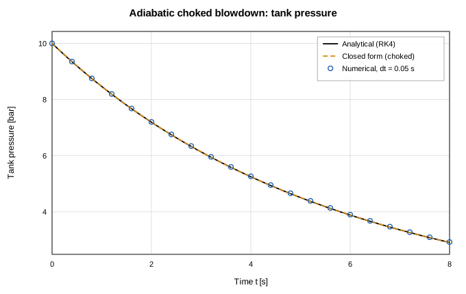
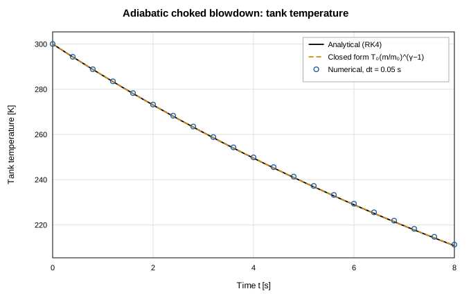
Figure 7-1 (top) and 7-2 (bottom). The adiabatic choked-blowdown verification case from docs/validation/tank-transient-report.md: tank pressure and temperature against the Runge–Kutta reference. The temperature trace is the signature of the internal-energy formulation — an isothermal model would be a horizontal line.

7.4 Water Distribution Network

Applications · steady · incompressible water

Problem. A pumped distribution tree serves three demand legs at different elevations.

Model. Eleven fluid nodes and twelve branches combining a pump, pipes, and elevation changes.

Check. The pump operates at the intersection of its curve and the system resistance, total delivered flow equals the sum of the legs, and the highest leg sees the lowest pressure. Raising one leg's elevation must reduce its flow. This example is the natural place to see how elevationChange sign conventions work in practice.

7.5 Heated Pipe with Radiating Wall

Applications · steady · incompressible water, conjugate

Problem. Water flows through a pipe whose wall is resolved as solid thermal mass, convecting to the fluid, conducting axially between wall segments, and radiating to a 300 K ambient.

Model. Four fluid nodes, three solid wall nodes, three branches, and five conductors spanning all three mechanisms.

Check. The global energy balance closes: heat radiated to ambient equals heat convected into the water plus any wall source. Wall temperatures fall monotonically along the flow direction. This is the smallest model that exercises conduction, convection, and radiation together, and it is the recommended template for a first conjugate model.

7.6 Spacecraft Radiator Panel (Ammonia Loop Heat Pipe)

Applications · steady · real-fluid ammonia, conjugate

Problem. An ammonia loop heat pipe rejects 400 W of avionics heat through a four-pass flat radiator panel to deep space.

Model. Twenty fluid nodes, twenty-three solid nodes, twenty branches, and sixty conductors. Capillary pumping in the wicked evaporator is represented as a fixed pump curve. The face sheet carries genuine two-dimensional in-plane conduction, and the panel is laid out in the x–y plane so the 3-D view is meaningful.

Check. Radiated heat matches the 400 W input at steady state. The two-dimensional conduction network spreads heat between passes, so face-sheet temperature varies in both directions — visible immediately with Color by set to Temperature. This example also demonstrates using View options to hide the sixty conductors while working on the flow path.

7.7 LOX/RP-1 Thruster (Combustor)

Applications · steady · mixed EOS, reacting junction, compressible duct, conjugate

Problem. A small regeneratively cooled LOX/RP-1 thruster: oxidizer and fuel feeds meet at a chamber, burn, and expand through a choked converging–diverging nozzle. Chamber pressure, mixture ratio, and product-gas properties are solved, not prescribed.

Model. Three circuits couple at a reacting junction (config.junctions; see combustion.md):

• LOX feed — tank → injector orifice → chamber;
• RP-1 feed — tank → 42-station counterflow regenerative jacket → injector orifice → chamber;
• hot gas — chamber → 42-station choked CD nozzle → exhaust, with momentumFlux and kineticEnergy on. The exhaust boundary is authored at the matched-expansion pressure, not an ambient pressure: a boundary node imposes a static pressure, and at a supersonic outlet any other value back-propagates into the last interior station.

The chamber energy row is the CEA closure $h = \eta\cdot h(T_0(P_c, O/F))$ with $\eta = 0.9409$. Every gas station carries a three-layer wall stack (inner liner, fins, outer shell) with film coefficients into its own RP-1 coolant node. Product-gas $R$, $\gamma$, $\mu$, and $c_p$ refresh from the same CEA lookup between outer Picard iterations.

Check. After Run, the chamber closes on $T = \eta\cdot T_0$ exactly. Injector mass flows match the orifice closed form against the solved chamber pressure. The nozzle chokes and the profile is monotone through the throat (the default limited-upwind faces, section 4.1.2). The three-layer wall stack matches the series–parallel resistance network. Full numbers and figures are in docs/validation/combustion-report.md. The formula-coupled twin (same feed/nozzle/jacket plumbing, but the chamber is an ordinary node fed by an imposed total mass flow instead of a reacting junction, and the coupling closes through an outer iteration instead of the monolithic Newton system) lands within about 1–2% on $P_c$ and the feed flows even when given the identical CEA-matched gas properties — the residual isolates the coupling architecture and discretization, not a mismatched gas assumption. See docs/validation/combustion-report.md for current numbers.

Scope. Requires kineticEnergy; frozen composition downstream of the chamber; standard-state reactant injection. The nozzle is perfectly expanded by construction — there is no shock capture (section 1.7). This example runs in steady mode; section 7.8 runs the same reacting junction transiently.

7.8 LOX/RP-1 Thruster (Transient Startup)

Applications · transient · mixed EOS, reacting junction, compressible duct

Problem. The same thruster as section 7.7, started up: LOX and RP-1 feed pressure ramps from 100 psi to 1000 psi over the first second and holds there for a second more (2 s total), while chamber pressure, mixture ratio, and product-gas properties evolve as the reacting junction fills.

Model. Reuses the geometry and thermal model of section 7.7's config.junctions chamber, feed lines, and 42-station regenerative jacket, with two changes: every fluid node (gas-path and coolant) is given a volume so its mass balance can integrate $d(\rho V)/dt$, and the LOX/RP-1 tank nodes carry a pressureSchedule ramp instead of a fixed pressure. The exhaust boundary is fixed at 30 kPa (a plausible high-altitude ambient) rather than sea-level, because at the low end of the ramp a sea-level boundary over-expands the nozzle enough to back-propagate an unphysical recompression kink into the last interior station; 30 kPa keeps the profile monotone at both ends of the ramp. settings.tolerance is relaxed to 1e-7 from the steady example's 1e-8, because the extra mass-storage row raises the raw residual's noise floor enough that the tighter bar is reachable only by grinding many extra inner-Newton iterations for no accuracy gain (outer-loop convergence is certified separately). See combustion.md for the full rationale.

Check. Chamber pressure rises monotonically during the ramp, lagging the feed-pressure schedule (the mass row's fill dynamic), then settles to a near-constant value during the hold (spread <0.01%). At every instant the chamber's temperature-vs-$P_c$ relationship still sits on the same steady CEA curve the energy closure enforces in section 7.7 — the energy row itself carries no storage term. The final held state matches a steady solve at the fully-ramped feed pressure to within 2% on $P_c$, $T_0$, and O/F. Full numbers and a figure of the pressure ramp are in docs/validation/combustion-report.md. The property panel's junction summary (Pc, O/F, mass flows, product-gas state) is indexed by the results timeline for this example, the same way it is scalar for section 7.7's steady run.

Scope. Same as section 7.7, plus: transient reacting junctions require a positive volume on the chamber node; the exhaust boundary is a fixed pressure chosen for this ramp's range rather than a matched-expansion value.

7.9 Water-Water Counterflow Heat Exchanger

Benchmarks · steady · incompressible water, conjugate

Problem. The counterflow heat exchanger of Example 5 in the GFSSP version 5 manual.

Model. Twenty-eight fluid nodes, twelve solid nodes, twenty-six branches, and twenty-four conductors, discretized at twelve passes.

Check. Published outlet temperatures are reproduced to 0.44 K on the hot side and 0.19 K on the cold side, with duty near 25.6 kW. This is the program's primary conjugate-heat-transfer benchmark against an independent code.

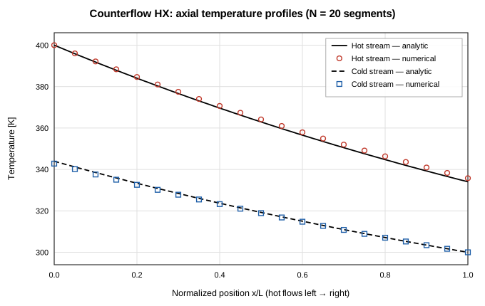
Figure 7-3. Axial temperature profiles from the thermal validation suite's counterflow heat-exchanger case, which mirrors the architecture of this example: per-segment wall solid nodes convecting to both streams. From docs/validation/thermal-network-report.md.

7.10 Entrapped-Air Line

Benchmarks · transient · incompressible water with gas cushion

Problem. The entrapped-air problem of Lee & Martin, reproduced as Figure 10 of the GFSSP manual: a water line closed by a pocket of trapped air oscillates after a valve operation.

Model. Twelve fluid nodes and eleven branches, with fluid inertia enabled on every pipe segment and a polytropic gas cushion on the downstream node.

Check. The first pressure peak is near 1.90 MPa, the oscillation period falls between 0.55 and 0.65 s, successive peaks decay, and the late-time mean approaches the reservoir pressure. The trace agrees with an independent fourth-order Runge–Kutta rigid-column reference to 8 % at a refined time step. This case is the joint test of inertia and gasCushion; disabling either one destroys the oscillation, which makes it a good demonstration of what those options actually do.

7.11 Cryogenic Line Cooldown

Benchmarks · transient · real-fluid hydrogen, conjugate

Problem. The C&R Technologies validation case drawn from NBS Report 9264, Figure 2 (Brennan et al., 1966): saturated liquid hydrogen at 75 psia is admitted to a 61 m copper line of 15.9 mm inside diameter, initially at 300 K, venting to 0.82 atm.

Model. Twenty axial segments — twenty-two fluid nodes, twenty solid nodes, twenty-one branches, and twenty convection conductors. Each segment carries a copper wall thermal mass with temperature-dependent NIST OFHC-copper specific heat and Miropolskii film-boiling convection. Fixed 1 s step.

Check. Walls chill sequentially from inlet to outlet — segment 1 well before segment 20 — and the first segment ends below 50 K. Chilldown time at the instrumented station is compared with the NBS experiment and with GFSSP predictions in the validation suite.

This is the most demanding shipped example: real-fluid two-phase flow, a moving front, temperature-dependent solid properties, and film boiling at once. It is also the clearest illustration of why axial discretization matters — a coarse version cannot resolve the front at all.

7.12 Extension: Cryo Tank Vent Control

Extensibility · transient · real-fluid nitrogen

Problem. A pressurized liquid-nitrogen ullage at about 3.2 bar takes a 400 W parasitic heat leak. A vent valve must hold pressure inside a band.

Model. Two fluid nodes and one branch, with logic rules opening and closing the vent on a 5 psi hysteresis band between P_high and P_low, while registers track ventOpen, peak pressure, and a vent-event count.

Check. Pressure cycles within the band, the valve state toggles at the thresholds, and the final register values report the peak pressure and number of vent events. This is the reference example for registers, logic rules, and hysteresis — the smallest complete demonstration of control without writing component code.

7.13 LH₂ Tank No-Vent Fill

Extensibility · transient · real-fluid parahydrogen, conjugate

Problem. SINDA/FLUINT Sample Problem F, model TVS: a half-full, saturated 42-inch liquid-hydrogen tank is filled from a colder 60 psia source while a thermodynamic vent system continuously bleeds liquid.

Model. Four fluid nodes, thirty-eight solid nodes, three branches, and sixty-nine conductors. FLUINT's twinned tanks and moveable ties have no schema equivalent here, so both are emulated from registers, logic rules, and register controllers: the liquid and vapor control volumes are boundary nodes whose pressure and temperature are integrated in logic and imposed each step, with densities and enthalpies read back from CoolProp parahydrogen, and nine wall ties reattach between the twins as the liquid level moves. The ullage is free to superheat, and a condensing film on each subcooled dry wall segment sets the condensation rate.

Check. At 15 minutes the model reproduces the reference deck within about 1 %: fill fraction 73.4 % against 73.9, pressure 59.63 psia against 59.72, vapor temperature 47.8 R against 47.4, and thermodynamic-vent flow 0.0518 lbm/hr against 0.0522.

Caveat. The vapor-cooled shield and internal heat exchanger are carried as solid thermal mass but are not resolved as flow paths — their ducts run at NTU ≈ 29 per node, beyond what the segregated solid-fluid coupling can solve. The module header of src/ui/lh2StorageTank.ts gives the full accounting. Read that before treating this example as a template.

7.14 Capillary Circuit (Stop + Trigger Valve)

Applications · transient · incompressible water, capillary channels

Problem. A capillary-driven ("capillaric") circuit with no pump: a sample wicks from a loaded inlet into a short channel A and a longer delay channel B that rejoin at a junction J, then through an outlet channel into a capillary pump that vents to atmosphere.

Model. Five nodes and five capillaryChannel branches (§4.3.19), all 100 µm × 50 µm except the pump. Channel A has 80° walls and a stop valve where it opens into J; B has 30° walls and twice A's length. The pump is a 1 mm-wide region represented by a 4 kPa capillaryPressure override. Only inlet is initiallyWet.

Check. The event log shows A's meniscus pinning at J (its Cho burst pressure is about 0.9 kPa and nothing supplies it), B wetting J about 45 ms later, and A being triggered at that same instant without bursting. The merged liquid then wets the pump inlet and the pump keeps wicking. All four circuit channels end full, with no airTrapped event.

Caveat. At the very start A briefly pins at its own entrance: B's faster front pushes air into J, and that gas back-pressure exceeds A's weak capillary pull for one step. This is real behaviour of a vented gas network, not an artefact.

7.15 Additional Configurations

Further networks are exported from the source tree but deliberately kept out of the menu, because they exist to be asserted on rather than explored: additional hand-checkable sanity cases (hydrostatic column, 50/50 flow split, equal-temperature mixing, tank equalization, conduction ladder with lumped cooldown), a pump-startup transient, a passive gas-cooled reactor loop, further GFSSP benchmark cases, single-phase and two-phase chilldown builders, and a nitrous-oxide cavitating venturi in steady and transient form. They are consumed by the validation suites in section 8 and by the research scripts under scripts/.

---

8. Verification and Validation

8.1 Approach

Verification here means three distinct things, and the distinction matters when citing a result. Analytic verification compares against a closed-form solution — the program should reproduce it to near machine precision, and any error is a code defect. Code-to-code benchmarking compares against another established program's published output; agreement supports the implementation but inherits the other code's assumptions. Validation against experiment compares against measured data; disagreement may be the model, the closure correlation, the discretization, or the experiment.

Cases in the following sections are labeled accordingly. Where a correlation is research-status or unvalidated, this manual says so rather than reporting an agreement figure.

8.2 Analytic Verification

Case	Reference	Tolerance
Hydrostatic column	$P = P_\text{top} + \rho g h$	10 Pa; zero flow
50/50 flow split	Half the source rate in each leg	0.001 kg/s
Orifice hand-calc	$C_d A\sqrt{2\rho\Delta P}$	0.5 %
Equal-temperature mixing	Flow-weighted mean temperature	0.05 K
Tank equalization	Volume-weighted mean pressure; mass conservation	300 Pa; 0.1 % mass
Conduction ladder and lumped cooldown	Linear profile; $\exp(-t/\tau)$	0.01 K; $\tau$ within 1 %
Multi-loop water network	Independent nodal Newton solution	0.5 % on branch flows
Pump-valve operating point	Bisection on the intersection	0.5 %
Coupled tank equalization	Runge–Kutta mass and energy integration	0.5 % pressure; 2 % trajectory
Heated-pipe temperature rise	Analytical cumulative heating	0.2 %
Tank blowdown	Runge–Kutta reference	2 % final pressure; 0.5 % discharged mass
Isentropic blowdown	$T/T_0 = (m/m_0)^{\gamma-1}$	1 %
Choked orifice	Analytical choked mass flux	0.5 %
Species decay	Exponential analytical solution	1 %
Adaptive stepping	Runge–Kutta reference on blowdown	2 %
Compressible duct flow, 5 cases	GFSSP TFAWS-2007 paper (NTRS 20070036728): Runge–Kutta integration of the generalized 1-D ODE; Fanno/Rayleigh closed forms. Full report with the paper's sixteen figures: docs/validation/compressible-report.md	Mass flow within 1 % (central scheme) / 2–6 % (default upwind); P, T, Mach profiles within 2–6 % (the paper's own 5 % band)
Real-fluid transonic CD nozzle	Analytic ideal-gas twin (same grid and scheme, N₂'s R and γ) plus the ideal choking relation; CoolProp nitrogen at 5 bar / 300 K (src/core/__tests__/realFluidTransonic.test.ts)	Mass flow within 0.17 % of the twin; chokes within the upwind margin; same root from a flat cold start
Reacting-junction LOX/RP-1 thruster	CEA identities; chamber and injector closed forms; quasi-1-D RK4 nozzle ODE; exact wall resistance network. Full report: docs/validation/combustion-report.md	Chamber closure to machine precision; injector error ≤0.18 %; local nozzle profile error ≤4.87 %; wall temperatures to machine precision
Two-phase HEM path	Nitrogen boiling and condensation staircases across the dome, and saturated LN₂ blowdown against a Runge–Kutta reference (src/core/__tests__/twoPhaseFlow.test.ts); the experimental leg is the NBS/GFSSP two-phase chilldown benchmark (section 8.4)	$T$ tracks $T_\text{sat}(P(t))$ within 0.5 K; pressure within 3 %; mass conserved to 0.5 %; latent-heat and flow-boiling energy balances within 1 %

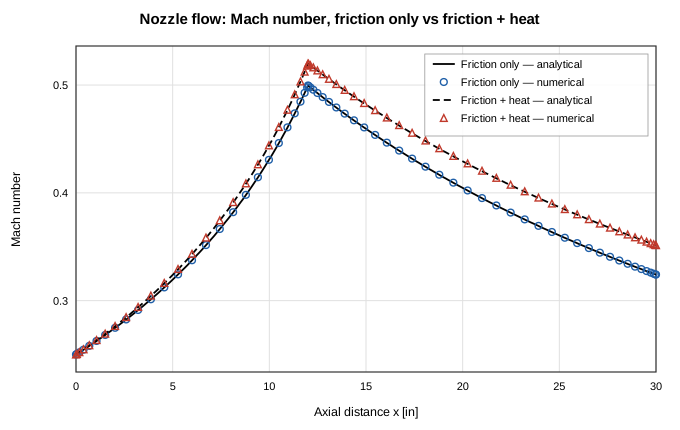
Figure 8-1. One of the sixteen figures from the compressible-duct validation report: Mach number along the TFAWS-2007 converging–diverging nozzle, friction-only and friction-plus-heat cases against the Runge–Kutta reference.

The remaining analytic families have their own generated reports, each regenerated from a live solve: incompressible hydraulics (docs/validation/incompressible-hydraulics-report.md), transient tanks (docs/validation/tank-transient-report.md), conjugate thermal networks (docs/validation/thermal-network-report.md), rigid-column fluid transients (docs/validation/fluid-transient-report.md), and reacting-junction combustion (docs/validation/combustion-report.md).

8.3 Code-to-Code Benchmarks

Benchmark	Reference	Result
GFSSP Example 13, conduction rod with convection	NASA/TM-2011-216470 §6.13	Solid temperatures within 3.0 K; conduction heat flows within 7 %; global energy balance within 0.5 %
N₂–N₂ counterflow heat exchanger	JANNAF 2024, Majumdar & LeClair	Duty within 5 %; outlet temperatures within 2.5 K; energy balance within 1 %
GFSSP Example 5, water-water heat exchanger	GFSSP v5 manual	Hot outlet 295.67 ± 1.0 K; cold outlet 290.94 ± 0.5 K; duty within 3 %
Lee & Martin entrapped air	GFSSP Figure 10; independent Runge–Kutta rigid column	First peak within 15 %; period 0.5–0.65 s; trace within 8 % at refined step
SINDA/FLUINT Sample F, LH₂ no-vent fill	C&R Technologies sample deck	Fill fraction, pressure, vapor temperature, and vent flow within about 1 % at 15 min
NURETH-16 gas-cooled reactor loop	NURETH-16 paper 13066	Published trends only; geometry is representative

8.4 Validation Against Experiment

The cryogenic chilldown corpus derives from NBS Report 9264. Table 6 of that report supplies eighteen chilldown-time points for saturated and subcooled liquid hydrogen and nitrogen, and eleven digitized oscillograph figures supply forty-four station traces totaling 10 195 samples, rebuilt from source CSVs by npm run gen:trace-corpus.

Corpus discipline is explicit about which data may be used for what. Four saturated runs, sixteen traces, are trusted and calibration-grade. Seven subcooled runs are diagnostic only: at coarse axial discretization their errors reach +80 %, so they may inform a diagnosis but may not be quoted as agreement. The continuous-integration chilldown baseline requires the computed chilldown time at the instrumented station to stay within a factor of 1.6 of experiment, with mean absolute error under 25 % across the full four-case slow suite. Two-phase chilldown energy and enthalpy balances close within 10 % and 12 % respectively.

Single-phase chilldown surrogates reproduce the qualitative plateau-then-plunge structure of the published figures but are not comparable on absolute times, and are asserted as trends only.

8.5 Correlation Status

Correlation	Source	Status
Swamee–Jain friction	Swamee & Jain (1976)	Standard explicit approximation
Dittus–Boelter	Dittus & Boelter (1930)	Standard; conductivity spot-checked against CoolProp within 3 %
Miropolskii film boiling	Miropolskii (1963) via Cross, Majumdar et al. (2002)	As used by GFSSP for chilldown; single-phase fallback to Dittus–Boelter
Darr–Hartwig	Darr & Hartwig (2020), NTRS 20190029114	Verified structurally against the published equations; fitted envelope is LH₂, vertical upflow, 1 g
TT-WF	In-tree design	Research status, not validated; transient-only
Custom expression	User-supplied	No published range; the user owns its validity
Solid property catalogue	NIST cryogenic, ANL-75-55, NASA/CR-2000-210055, and others	Per-material validity ranges with end-value clamping; see docs/solid-properties-results.md

8.6 Test Tiers

Command	Scope
npm test	Fast pull-request tier; excludes expensive scientific suites
npm run check	Production build plus the fast tier
npm run test:all	Every Vitest file, with opt-in slow blocks still skipped
npm run test:slow	Adds the opt-in slow scientific validation blocks
npm run test:e2e	Playwright suite against a production preview build

Tier composition and the rationale for each opt-in block are documented in docs/testing-slow.md.

8.7 Result Provenance

Every run hashes the configuration that produced it. Results computed from a model that has since been edited are marked stale beside the run title, in the property panel, and on the canvas, and the interface says plainly that a stale number should be rerun before it informs a decision. Sweep jobs freeze and hash their snapshot at creation, so a later edit raises a staleness banner instead of silently changing the basis of a comparison. Channel exports, table exports, sweep CSVs, and solver diaries all carry the model name, a solver-settings summary, and the config hash.

Notes are excluded from the hash by design, so documenting a model never invalidates a run.

---

Appendix A — Branch Component Quick Reference

Interface labels are grouped Common, Advanced, and Custom in the Component Type selector. All areas are m², lengths m, pressures Pa.

type	Label	Parameters	Relation	Restrictions
pipe	Pipe	length, diameter, roughness, elevationChange?, inertia?, frictionFactor?, diameterOut?	§4.3.1	inertia transient-only
valve	Valve	area, cd, position, positionSchedule?	§4.3.6	position on [0,1]
orifice	Orifice	area, cd	§4.3.2	$Y(r,\kappa)$ from the branch fluid; chokes when $r < r_*$
pump	Pump	curve as $(Q,\Delta P_\text{rise})$ pairs	§4.3.10	rise must decrease monotonically
checkValve	Check Valve	area, cd	§4.3.7	—
dynamicCheckValve	Dynamic Check Valve	area, cd, discArea?, mass, springRate, preload, damping, stroke, initialPosition?	§4.3.8	mass, springRate, stroke > 0; initialPosition on [0,1]
reliefValve	Relief Valve	crackPressure, fullOpenPressure, area, cd	§4.3.9	full-open > crack
flowSource	Flow Source	massFlow, massFlowSchedule?	§4.3.13	—
cavitatingVenturi	Cavitating Venturi	throatArea, cd, recoveryFactor?	§4.3.3	requires realFluid
resistance	Resistance	k, area	§4.3.5	$k \ge 0$
bend	Bend	diameter, angle, rOverD, roughness?	§4.3.11	angle on (0,180]
areaChange	Area Change	areaIn, areaOut	§4.3.12	both positive
regulator	Regulator	setPressure, maxCdA	§4.3.14	both positive
heatedPipe	Heated Pipe	pipe fields plus ua, wallTemperature, boilingModel?	§4.3.15	$UA \ge 0$
dpTable	Pressure Drop Table	points, extrapolate?	§4.3.16	≥2 points, $\dot m$ increasing
customResistance	Custom Resistance	k or {kTable}, area, diameter?	§4.3.5	kTable requires diameter
rectChannel	Rectangular Channel	width, height, length, roughness?, elevationChange?	§4.3.18	dimensions positive
capillaryChannel	Capillary Channel	rect fields, contactAngle (+ per-wall), surfaceTension?, stopValve?, initialFill?, …	§4.3.19	incompressible fluid; angles on [0,180]
userComponent	Local Component	component, params?, area?	§4.3.17	must exist in the library

Appendix B — Conductor Quick Reference

kind	Label	Parameters	Relation	Endpoints
conduction	Conduction	k, area, length	$\dot Q = \dfrac{kA}{L}\Delta T$	both thermal
convection	Convection	area, h or correlation	$\dot Q = h_c A \Delta T$	one fluid, one thermal
radiation	Radiation	emissivity, area, viewFactor	$\dot Q = \varepsilon\sigma A F \Delta(T^4)$	both thermal

Convection correlation.model accepts dittusBoelter, miropolskii, darrHartwig (needs axialPosition), ttWf (needs axialPosition and segmentLength; transient-only), or custom (needs expression). All named models require realFluid.

Appendix C — The .fn File Format

A saved model is a line-oriented text projection of the canonical NetworkConfig, not JSON, though the same schema is accepted as JSON internally for browser autosave. The projection is lossless and includes groups, notes, variants, and node group membership. A file with no variants serializes identically to one written before the field existed.

header       ::= "// Fluid Network config v2"
networkLine  ::= "network " jsonString " {"
nodeRec      ::= "node " jsonString " " nodeType
                 " @ (" num ", " num [", " (num | "null")] ") data: " jsonObject
branchRec    ::= "branch " jsonString ": " jsonString " -> " jsonString
                 " " componentType " data: " jsonObject
conductorRec ::= "conductor " jsonString ": " jsonString " -> " jsonString
                 " " conductorKind " data: " jsonObject

One record per line with LF newlines. Values are read and written with JSON.parse and JSON.stringify only — never evaluated. Numbers are always SI; a unit preset may appear but is ignored on load. Empty optional collections are written explicitly so that a round trip is byte-stable.

A record's data object carries every field not already on the record line. For a branch that is { label?, initialMdot?, ...component fields except type }, so the Newton mass-flow warm start that central-scheme near-choked compressible ducts require (and that remains a useful convenience under the default upwind scheme) survives a save/load cycle along with the model geometry.

Parsing never throws. It returns diagnostics with line numbers, and a file that fails to parse never replaces the current network. After parsing, the result goes through the same decode and validation pipeline as any other input (section 5.2). The implementation is src/substrate/textProjection.ts.

Appendix D — Glossary

Adaptive stepping — Time-step control by local error estimation through step doubling.

Ambient node — Fixed-temperature thermal reservoir of unbounded capacity.

Boundary node — Fluid node with imposed pressure and temperature; an infinite reservoir that anchors the network's pressure level.

Branch — Directed connection between two fluid nodes carrying one mass flow unknown.

Channel — A named scalar time series or steady value in a result, the unit of selection and export in the Results view.

Conductor — Directed thermal link carrying heat by conduction, convection, or radiation.

Config hash — Fingerprint of the model that produced a result, used to detect staleness. Excludes notes.

Conjugate heat transfer — Simultaneous solution of fluid and solid energy with implicit coupling at their interface.

Gas cushion — Trapped compressible gas volume in a liquid node, obeying $PV_g^n = \text{const}$.

Globalization — Strategy ensuring a Newton step reduces the residual; trust-region dogleg or backtracking line search.

HEM — Homogeneous equilibrium model; two-phase mixture treated as a single fluid in thermodynamic equilibrium.

Internal node — Fluid node whose pressure and temperature are solved.

Momentum flux — Optional convective acceleration term in branch momentum.

PTC — Pseudo-transient continuation; regularization of a steady Newton solve by an artificial time term that vanishes at convergence.

Solid node — Lumped thermal mass with finite capacity $m c_p$.

Solver diary — Bounded, provenance-carrying record of a run's convergence history.

Stale result — A result whose model has been edited since the run.

Subnetwork (group) — Visual container with no effect on results.

Upwinding — Taking a convected property from the upstream node according to the sign of the mass flow.

Variant — A named sparse patch over the base network, stored in the .fn file as config.variants. The solver never sees variants; the editor resolves the active one first. Runs are filed under the variant that produced them.

Appendix E — References

1. Majumdar, A. K., LeClair, A. C., Moore, R., and Schallhorn, P. A., Generalized Fluid System Simulation Program, Version 6.0, NASA/TM-2013-217492, Marshall Space Flight Center, October 2013. https://ntrs.nasa.gov/citations/20140003178
2. Generalized Fluid System Simulation Program (GFSSP), Supplementary Documentation for Version 701, NASA, 2024.
3. Majumdar, A. K., and LeClair, A. C., conjugate heat-exchanger modeling with GFSSP, JANNAF, 2024.
4. Brennan, J. A., et al., Cooldown of Cryogenic Transfer Lines, NBS Report 9264, National Bureau of Standards, 1966.
5. Cross, M. F., Majumdar, A. K., et al., "Modeling of Chill Down in Cryogenic Transfer Lines," Journal of Spacecraft and Rockets, Vol. 39, No. 2, 2002.
6. Darr, S. R., and Hartwig, J. W., "Optimal liquid nitrogen and liquid hydrogen chilldown correlations," Cryogenics, Vol. 105, 102999, 2020. NTRS 20190029114.
7. Dittus, F. W., and Boelter, L. M. K., University of California Publications in Engineering, Vol. 2, 1930, p. 443.
8. Miropolskii, Z. L., "Heat transfer in film boiling of a steam-water mixture in steam-generating tubes," Teploenergetika, Vol. 10, No. 5, 1963.
9. Swamee, P. K., and Jain, A. K., "Explicit equations for pipe-flow problems," Journal of the Hydraulics Division, ASCE, Vol. 102, No. 5, 1976.
10. Ellis, D. L., Thermophysical Properties of GRCop-84, NASA/CR-2000-210055, 2000. https://ntrs.nasa.gov/citations/20000064095
11. Idelchik, I. E., Handbook of Hydraulic Resistance, 3rd ed., 1994.
12. Crane Co., Flow of Fluids Through Valves, Fittings, and Pipe, Technical Paper No. 410.
13. Bell, I. H., Wronski, J., Quoilin, S., and Lemort, V., "Pure and Pseudo-pure Fluid Thermophysical Property Evaluation and the Open-Source Thermophysical Property Library CoolProp," Industrial & Engineering Chemistry Research, Vol. 53, No. 6, 2014, pp. 2498–2508.
14. SINDA/FLUINT User's Manual, C&R Technologies.
15. Bandyopadhyay, A., and Majumdar, A., "Modeling of Compressible Flow with Friction and Heat Transfer using the Generalized Fluid System Simulation Program (GFSSP)," TFAWS 2007, MSFC-464, NTRS 20070036728. https://ntrs.nasa.gov/citations/20070036728

Companion Documentation

Document	Contents
README	Project overview, quick start, and documentation index
Architecture	Module boundaries, APIs, configuration lifecycle
User extensibility	User components, registers, logic, controllers, trust model
Parameter bindings	Formula-bound fields, convection models, solid property models
Solver convergence	Known convergence behavior
Real-fluid performance	CoolProp backend, derivatives, performance
Fluid catalogue	124-fluid CoolProp catalogue
Solid properties	Material catalogue sources and validation
Fluid-front transport	Front transport model and verification
Combustion	CEA-coupled reacting junctions, table generation, and model limitations
Testing tiers	Fast, all-files, and slow validation commands
Compressible duct-flow validation	NASA GFSSP TFAWS-2007 recreation: five cases, sixteen figures
Combustion validation	CEA identities, chamber/injector closure, nozzle profiles, and regenerative wall stack
Incompressible hydraulics validation	Closed-form pipe hydraulics: Hagen–Poiseuille, Darcy–Weisbach, Hardy-Cross, hydrostatics, pump operating point
Transient tank validation	Lumped tank gas dynamics: blowdown, equalization, fill heating
Thermal network validation	Composite wall, radiation–convection equilibrium, lumped cooldown, heated pipe, ε–NTU HEX
Rigid-column fluid-transient validation	Lumped inertia and gas cushion vs rigid-column surge theory
Microfluidics validation	Rectangular-duct and capillary closures vs exact solutions; six published microfluidic networks