
Thermal Network and Conjugate Heat Transfer Validation of OpenFLUME
Analytic verification of the solid-node thermal system — conduction, convection, and radiation conductors — and of its conjugate coupling to the fluid network
Generated by scripts/thermal-validation-report.ts — all numbers and figures come from live solves of the current solver. The corresponding CI gates are src/core/__tests__/thermal.test.ts and src/core/__tests__/solidThermalTransient.test.ts.
Abstract
This report verifies the conjugate thermal capability of the OpenFLUME solver — a pressure-based node-and-branch network code in the same family as NASA's GFSSP — against classical closed-form heat-transfer solutions. Five benchmark cases exercise every conductor kind and both coupling directions between the solid and fluid systems: a steady composite plane wall (series thermal-resistance network), the nonlinear radiation–convection equilibrium of a heated solid node, the lumped-capacitance transient cooldown, a heated pipe approaching a constant wall temperature, and — the flagship case — a counterflow heat exchanger of two water streams wall-coupled through solid nodes, compared against the ε–NTU closed form. The steady resistance-network cases reproduce the analytic solutions to near machine precision (composite-wall heat flow within 6.9e-14 %, radiation equilibrium temperatures within 1.2e-14 %); the transient cooldown follows the exponential within 0.18 % of the temperature span at dt = τ/100 and exhibits the expected first-order time-step convergence of backward Euler (error ratio 4.01 for a 4× step refinement); the heated pipe reproduces the exponential wall-temperature approach to 1.8e-14 %; and the 20-segment heat exchanger predicts effectiveness within 2.62 % and both outlet temperatures within 1.730 K of the ε–NTU solution, with the residual discrepancy shown to be finite-segmentation error that vanishes monotonically as the wall discretization is refined.
Introduction
Fluid-network codes that carry only fluid unknowns cannot represent hardware thermal mass, structural conduction paths, or radiation sinks — all of which dominate problems like cryogenic line chilldown, heat-exchanger sizing, and thermal protection. OpenFLUME therefore carries a second, thermal network alongside the fluid one: solid nodes with optional thermal capacitance (mass × cp) and prescribed heat inputs, ambient nodes at fixed temperature, and conductors of three kinds — conduction (kA/L), convection (hA, attaching a solid to a fluid node), and radiation (σεAF between solid/ambient nodes). Heated-pipe branches provide a complementary lightweight fluid heating path against a prescribed wall temperature. The purpose of this report is to verify that machinery the same way the compressible-flow capability was verified (see docs/validation/compressible-report.md): live solves of small networks against independent analytic references, with every number in this document interpolated from those solves.
Problem Description
Five cases cover the three conductor kinds, both steady and transient solid physics, and both directions of conjugate coupling (fluid heating a wall, walls heating a fluid):
| Case | Description | Reference |
|---|---|---|
| 1 | Steady composite plane wall: convection–conduction–conduction–convection in series | Resistance sum, Q = ΔT/ΣR |
| 2 | Radiation–convection equilibrium of a solid node with fixed heat input, swept over q | Newton root-solve of the T⁴ balance |
| 3 | Lumped-capacitance transient cooldown by convection, two time steps | T(t) = T∞ + (T₀−T∞)e^(−t/τ) |
| 4 | Heated pipe: 10 constant-wall-temperature segments in series | Exponential axial approach |
| 5 | Counterflow heat exchanger: two water streams wall-coupled per segment | ε–NTU closed form |
Composite Wall
Case 1 is the classic two-layer furnace wall (Figure 1): hot fluid at 500 K with film coefficient h₁ = 40 W/m²K, a 10 cm layer of k₁ = 1.2 W/mK, a 5 cm layer of k₂ = 0.05 W/mK, and cold fluid at 300 K with h₂ = 10 W/m²K, over A = 1 m². Three solid nodes sit at the two surfaces and the layer interface; the two fluids are boundary nodes of the fluid network.

Figure 1. Composite wall: three solid nodes (surfaces and interface), two conduction and two convection conductors between two fluid boundary nodes.
Counterflow Heat Exchanger
Case 5 mirrors the architecture of GFSSP Example 5 (the water–water counterflow heat exchanger, user manual §7.9): each axial segment carries an internal fluid node on the hot stream, an internal fluid node on the cold stream, and a wall solid node between them, with convection conductors on both faces (Figure 2). The hot stream (0.2 kg/s, 400 K in) flows left to right; the cold stream (0.3 kg/s, 300 K in) flows right to left. Both film coefficients are 500 W/m²K over a total transfer area of 5 m² per side, so the overall conductance UA = hA/2 = 1250 W/K is independent of the segment count and the segment sweep isolates pure discretization error. The capacity rates are deliberately unequal (C_r = 0.6667) to exercise the general ε–NTU form rather than the degenerate balanced case.

Figure 2. Counterflow heat exchanger: per-segment wall solid nodes with convection conductors to both streams, mirroring GFSSP Example 5.
Benchmark Solutions
Series resistance network (case 1). In steady state the heat flow through every element of the chain is equal, so the wall behaves as resistances in series:
$$\Sigma R = \frac{1}{h_1 A} + \frac{L_1}{k_1 A} + \frac{L_2}{k_2 A} + \frac{1}{h_2 A}, \qquad \dot Q = \frac{T_{\infty 1} - T_{\infty 2}}{\Sigma R},$$
and the surface and interface temperatures follow from partial sums, $T_{s,i} = T_{\infty 1} - \dot Q \sum_{j \le i} R_j$. With the case-1 numbers, ΣR = 1.208333 K/W and Q̇ = 165.5172 W.
Radiation–convection equilibrium (case 2). A solid node with heat input q losing to a common sink temperature T∞ by convection and radiation settles where
$$q = hA,(T - T_\infty) + \sigma \varepsilon A F,(T^4 - T_\infty^4).$$
The quartic has one physical root above T∞; the reference is a Newton iteration on this balance, converged to 10⁻¹² K in-script.
Lumped capacitance (case 3). A solid of thermal capacitance mc cooling through a convection conductance hA obeys
$$m c \frac{dT}{dt} = -hA,(T - T_\infty) ;\Rightarrow; T(t) = T_\infty + (T_0 - T_\infty),e^{-t/\tau}, \qquad \tau = \frac{mc}{hA}.$$
For the physical problem this classical solution requires a small Biot number (Bi = hL_c/k ≲ 0.1) so the solid is spatially isothermal; for the network model the comparison is exact by construction, because a solid node is a lumped capacitance with no internal resistance — which makes this a pure test of the time integrator.
Heated pipe with constant wall temperature (case 4). A fluid stream ṁcp exchanging with a fixed wall temperature through a uniformly distributed conductance UA obeys dT/dx = (UA/L)(T_w − T)/(ṁc_p), giving the exponential approach
$$T(x) = T_w - (T_w - T_{in}),\exp\left(-\frac{UA}{\dot m c_p}\frac{x}{L}\right).$$
The solver's heated-pipe branch applies exactly the per-segment effectiveness form ε = 1 − exp(−UA_seg/ṁc_p), whose composition over equal segments reproduces this exponential at every node; the comparison therefore isolates the branch heat-delivery path and the coupled energy balance rather than a discretization error.
Counterflow ε–NTU (case 5). With NTU = UA/C_min and C_r = C_min/C_max, the counterflow effectiveness is
$$\varepsilon = \frac{1 - \exp\left(-\mathrm{NTU},(1 - C_r)\right)}{1 - C_r \exp\left(-\mathrm{NTU},(1 - C_r)\right)},$$
and the outlet temperatures follow from q = εC_min(T_{h,in} − T_{c,in}). The axial profiles come from the temperature-difference ODE dΔT/dx = −(UA/L)(1/C_h − 1/C_c)ΔT, whose exponential solution is anchored by the ε–NTU outlet states (cross-checked in-script to 10⁻⁹ K). With the case-5 numbers, NTU = 1.4945, C_r = 0.6667, and ε = 0.6595.
Numerical Modeling
The thermal network adds one temperature unknown per solid node. Each solid node enforces an energy balance over its attached conductors and prescribed heat input,
$$m c_p \frac{dT_i}{dt} = \sum_j \dot Q_{ji} + \dot Q_{input,i},$$
with the storage term dropped in steady mode (and the backward-Euler form m c_p (T_i^{n+1} − T_i^n)/Δt in transient mode — first-order in time). The conductor heat rates take the three classical forms: conduction Q̇ = (kA/L)(T_i − T_j), convection Q̇ = hA(T_s − T_f) against a fluid-node temperature, and radiation Q̇ = σεAF(T_i⁴ − T_j⁴) between solid/ambient nodes. The solid temperatures are solved as a segregated thermal subsystem by a Newton iteration with an exact analytic Jacobian — including the 4σεAFT³ radiation derivative, which is what lets the strongly nonlinear case-2 balance converge from a cold start (the Jacobian is verified entry-by-entry against central finite differences in src/core/__tests__/solidThermalTransient.test.ts).
Conjugate coupling runs in both directions. Convection conductors deposit their heat rate into the attached fluid node's energy balance, so a heated wall raises the downstream fluid temperature through the ordinary advective energy equation; conversely the fluid temperature enters the conductor's driving ΔT. Heated-pipe branches short-cut this when the wall temperature is known rather than solved: they deliver Q̇ = ṁc_pε(T_w − T_in) with ε = 1 − exp(−UA/ṁc_p) directly to the downstream node. In cases 1–3 the fluid network is reduced to boundary nodes (fixed T∞ reservoirs) with a zero-flow source branch, mirroring the CI-test configurations; in cases 4–5 the streams carry real through-flow (case 4 pressure-driven through an orifice, case 5 imposed by flow sources on both streams, exactly as in the CI heat-exchanger test).
In the segmented heat-exchanger model each stream's internal node holds its cell-outlet state (an implicit upwind discretization of the counterflow ODEs), so hot node i is plotted at x = i/N and cold node i — flowing right to left — at x = (i−1)/N. The scheme is first-order in the segment width, which is the discretization error the segment sweep of Figure 8 quantifies.
Results and Discussion
| Case | Compared quantity | Max deviation | Notes |
|---|---|---|---|
| 1 — composite wall | heat flow Q̇ | 6.9e-14 % | series chain spread 6.0e-13 % |
| 1 — composite wall | surface/interface T (3 nodes) | 0.00e+0 K (0.0e+0 %) | near machine precision |
| 2 — radiation–convection | equilibrium T over 6-point q sweep | 1.2e-14 % | balance residual ≤ 2.3e-14 % of q |
| 3 — lumped transient (dt = τ/25) | T(t) vs exponential | 0.72 % of span | backward Euler, first order |
| 3 — lumped transient (dt = τ/100) | T(t) vs exponential | 0.18 % of span | error ratio 4.01 vs 4 expected |
| 4 — heated pipe (10 segments) | axial T profile, 10 nodes | 1.8e-14 % | outlet within 5.68e-14 K |
| 5 — counterflow HX (N = 20) | effectiveness ε | 2.62 % | outlets within 1.730 K; segmentation error, first order in 1/N |
Case 1: Composite Plane Wall
The solver reproduces the series-resistance solution essentially exactly: Q̇ = 165.5172 W against the analytic 165.5172 W (6.9e-14 %), with the same heat flow through all four elements of the chain to 6.0e-13 % — the discrete statement that the steady resistances are truly in series. The hot-surface, interface, and cold-surface temperatures are 495.86 K, 482.07 K, and 316.55 K against analytic values of 495.86 K, 482.07 K, and 316.55 K — a worst deviation of 0.00e+0 K (Figure 3). The insulation layer carries 82.8 % of the total resistance and correspondingly almost the entire temperature drop, a useful visual check that each conductor carries its intended share.

Figure 3. Temperature through the composite wall: analytic piecewise-linear profile and solver solid-node temperatures; dashed levels are the two fluid reservoir temperatures.
Case 2: Radiation–Convection Equilibrium
A solid node with fixed heat input q sheds it through a convection conductor (h = 15 W/m²K, A = 0.05 m²) to a 300 K fluid and a radiation conductor (ε = 0.8, A = 0.05 m², F = 1) to a 300 K ambient. Sweeping q from 100 to 4000 W moves the equilibrium from 388.8 K to 1107.5 K, across which the radiated share of the load grows from 33.4 % to 84.9 % — the sweep genuinely crosses from convection-dominated to radiation-dominated territory. The solver matches the Newton reference within 1.2e-14 % at every point (Figure 4, Table below), and substituting the solver temperatures back into the analytic balance leaves a residual below 2.3e-14 % of q, confirming the exact treatment of the T⁴ conductor in the thermal Newton system.
| q [W] | T_eq analytic [K] | T_eq solver [K] | deviation |
|---|---|---|---|
| 100 | 388.755 | 388.755 | 0.0e+0 % |
| 250 | 487.300 | 487.300 | 1.2e-14 % |
| 500 | 599.786 | 599.786 | 0.0e+0 % |
| 1000 | 741.854 | 741.854 | 0.0e+0 % |
| 2000 | 910.723 | 910.723 | 1.2e-14 % |
| 4000 | 1107.535 | 1107.535 | 0.0e+0 % |
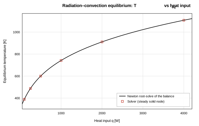
Figure 4. Equilibrium temperature vs heat input: Newton root-solve of the convection + radiation balance (line) and steady solver results (markers).
Case 3: Lumped-Capacitance Transient Cooldown
A solid node (m = 1 kg, c_p = 500 J/kg·K) initially at 400 K cools through a convection conductor (hA = 10 W/K) to a 300 K reservoir; τ = mc_p/hA = 50 s. Two fixed time steps were run to 3τ. At dt = τ/25 = 2 s the trace deviates from the exponential by at most 0.72 % of the 100 K span (|ΔT| = 0.724 K at τ, 0.300 K at 3τ); refining to dt = τ/100 = 0.5 s reduces the 3τ error to 0.0747 K — a ratio of 4.01 for a 4× step refinement, consistent with the first-order accuracy of backward Euler (Figure 5). The integrator is unconditionally stable and monotone here, so the choice of dt is purely an accuracy trade, not a stability one.
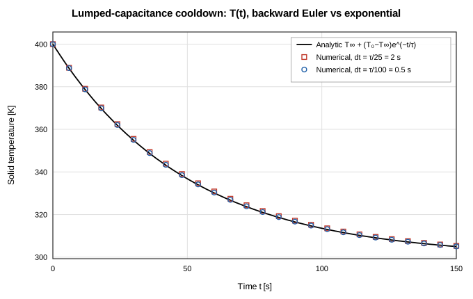
Figure 5. Lumped-capacitance cooldown: analytic exponential and backward-Euler traces at dt = τ/25 and dt = τ/100 (markers subsampled for legibility).
Case 4: Heated Pipe with Constant Wall Temperature
Water enters 10 series heated-pipe segments (D = 0.02 m, L = 2 m total, UA = 250 W/K per segment) at 300 K with the wall held at 350 K; the flow is pressure-driven and the solved rate is ṁ = 0.36218 kg/s, giving a total NTU = 1.651 and an expected outlet approach of ε = 80.8 % of the wall–inlet difference. The axial profile follows the analytic exponential at all 10 nodes to within 1.8e-14 %, with the outlet at 340.403 K against the analytic 340.403 K (Figure 6). Agreement at this level is expected rather than remarkable — the branch model applies the same per-segment effectiveness relation the analytic solution composes — but it verifies the heat-delivery path into the downstream node energy balance and the coupled solve of flow rate and temperature, with the reference evaluated at the solved ṁ exactly as in the CI test.
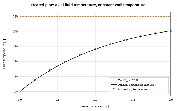
Figure 6. Heated pipe: analytic exponential approach to the wall temperature and solved node temperatures along the pipe string.
Case 5: Counterflow Heat Exchanger (flagship)
The 20-segment exchanger predicts ε = 0.6422 against the ε–NTU value of 0.6595 — a deviation of 2.62 % — with outlet temperatures of 335.78 K (hot) and 342.82 K (cold) against analytic values of 334.05 K and 343.97 K (deviations of 1.730 K and 1.153 K). The hot- and cold-side duties agree to 1.7e-5 %, confirming that the wall nodes store nothing in steady state and simply relay the heat. The axial profiles (Figure 7) track the analytic exponentials within 1.730 K everywhere on both streams.
The residual effectiveness error is finite segmentation, not physics: each segment lumps its exchange at the cell-outlet states (implicit upwind), which under-predicts the local ΔT and hence the duty. Because total UA is held fixed as the segment count varies, the sweep of Figure 8 isolates that error: the numerical effectiveness rises monotonically toward the closed form, from 21.26 % low at N = 2 to 1.89 % at N = 28, with the error falling roughly in proportion to 1/N as expected of a first-order scheme. This is the same segmentation trade GFSSP documents for its Example 5 model, which uses twelve passes.
| N segments | ε numerical | ε deviation | T_h,out [K] | T_c,out [K] | hot/cold duty imbalance |
|---|---|---|---|---|---|
| 2 | 0.5193 | 21.26 % | 348.07 | 334.62 | 7.6e-6 % |
| 3 | 0.5590 | 15.24 % | 344.10 | 337.27 | 9.7e-6 % |
| 5 | 0.5953 | 9.73 % | 340.47 | 339.69 | 9.5e-6 % |
| 8 | 0.6179 | 6.31 % | 338.21 | 341.19 | 9.1e-6 % |
| 12 | 0.6312 | 4.30 % | 336.88 | 342.08 | 1.2e-5 % |
| 16 | 0.6380 | 3.26 % | 336.20 | 342.54 | 1.5e-5 % |
| 20 | 0.6422 | 2.62 % | 335.78 | 342.82 | 1.7e-5 % |
| 28 | 0.6471 | 1.89 % | 335.29 | 343.14 | 2.2e-5 % |
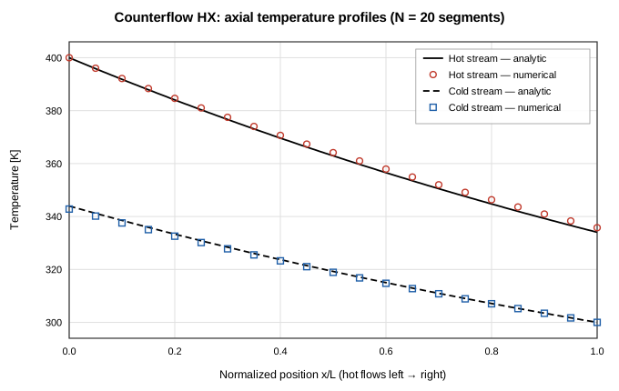
Figure 7. Counterflow HX axial temperature profiles at N = 20: analytic (lines) vs numerical node temperatures (markers), hot stream flowing left to right, cold stream right to left.
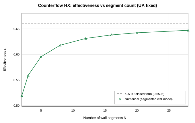
Figure 8. Effectiveness vs segment count at fixed total UA: monotone first-order approach of the segmented wall model to the ε–NTU closed form.
Conclusions
The thermal-network machinery of OpenFLUME — solid and ambient nodes, conduction, convection, and radiation conductors, heated-pipe branches, and the segregated exact-Jacobian thermal Newton subsystem — reproduces the five classical benchmarks. Steady resistance-network problems solve to near machine precision (6.9e-14 % on composite-wall heat flow, 1.2e-14 % on radiation–convection equilibria across a q sweep that moves the radiated share from 33.4 % to 84.9 % of the load). The backward-Euler transient integrator follows the lumped-capacitance exponential within 0.72 % of span at dt = τ/25 and converges at first order, its documented accuracy. Conjugate coupling is verified in both directions: heated-pipe branches reproduce the exponential wall-temperature approach to 1.8e-14 %, and the wall-coupled counterflow heat exchanger matches ε–NTU effectiveness within 2.62 % at twenty segments, with the remaining discrepancy demonstrated to be first-order segmentation error that shrinks monotonically under refinement. Known limitations follow directly from the formulation: transient accuracy is first order in Δt, and segmented heat-exchanger duty converges from below at first order in 1/N, so segment count should be chosen against the NTU per segment rather than by habit.
References
- Incropera, F. P., DeWitt, D. P., Bergman, T. L., and Lavine, A. S., Fundamentals of Heat and Mass Transfer, 6th ed., John Wiley & Sons, 2007 (composite walls, lumped capacitance, radiation exchange, ε–NTU).
- Kays, W. M., and London, A. L., Compact Heat Exchangers, 3rd ed., McGraw-Hill, 1984 (effectiveness–NTU relations for counterflow).
- Majumdar, A. K., LeClair, A. C., Moore, R., and Schallhorn, P. A., Generalized Fluid System Simulation Program, Version 6.0, NASA/TM-2013-217492, 2013 (Example 5: water–water counterflow heat exchanger; conjugate solid–fluid formulation).
Nomenclature
| Symbol | Meaning |
|---|---|
| A | heat-transfer area |
| Bi | Biot number hL_c/k |
| C | capacity rate ṁc_p |
| C_r | capacity ratio C_min/C_max |
| c_p | specific heat |
| F | radiation view factor |
| h | convective film coefficient |
| k | thermal conductivity |
| L | thickness / length |
| m | solid node mass |
| ṁ | mass flow rate |
| NTU | number of transfer units UA/C_min |
| Q̇, q | heat rate / heat input |
| R | thermal resistance |
| T | temperature |
| T∞ | reservoir (fluid or ambient) temperature |
| UA | overall conductance |
| ε | heat-exchanger effectiveness; radiation emissivity |
| σ | Stefan–Boltzmann constant |
| τ | lumped-capacitance time constant mc_p/hA |